Adding numbers in Google Sheets looks simple until the sheet grows beyond a few cells. A quick + formula works for a small row total, but it becomes fragile when you need to total a range, include separate areas, pull values from other tabs, or count only records that meet a rule.

The right Google Sheets adding formula depends on how your data is arranged. Start with the simplest option that fits the job, and your spreadsheet will be much easier to update later.

Choose the right Google Sheets adding formula

Every formula in Google Sheets starts with an equals sign (=). Once a formula references cells rather than typed-in numbers, it recalculates automatically whenever those source values change.

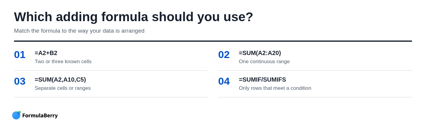
Use these defaults:

• Use =A2+B2 for two or three known cells.
• Use =SUM(A2:A20) for one continuous range.
• Use =SUM(A2,A10,C5) for separate cells or ranges.
• Use SUMIF or SUMIFS when only rows matching a condition should be included.

Add individual cells with the plus sign

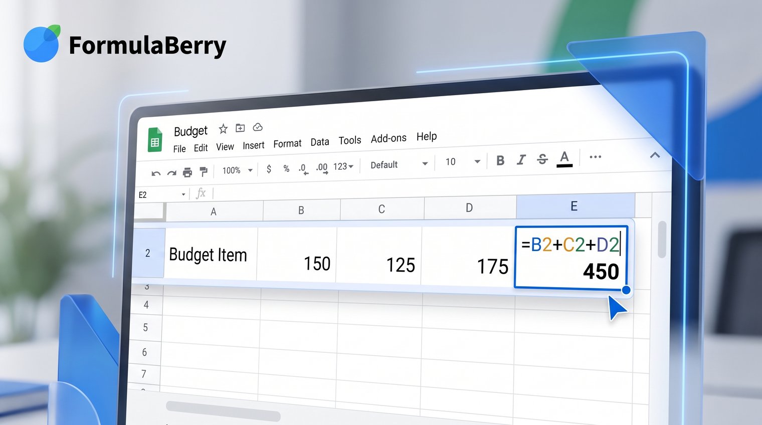
For a short row of values, use the plus sign. If an invoice has an item amount in B2, tax in C2, and shipping in D2, enter this in the total cell:

=B2+C2+D2

Google Sheets adds the current values in those cells. Change the tax or shipping amount later, and the total updates without any extra work.

This is a good Google Sheets add formula for a compact calculation you can read at a glance. It is not the best choice for 10, 20, or 100 cells. A long chain such as =B2+C2+D2+E2+F2+G2 is difficult to inspect and easy to break. Switch to SUM when the cells form a range.

Use cell references instead of typing the numbers

Prefer =A2+B2 over =10+25. The first formula stays connected to your sheet; the second is permanently fixed at 35 until you edit the formula itself.

To reduce typing mistakes, click the result cell, type =, click the first cell, type +, then click the next cell. Google Sheets inserts the references for you. Press Enter when the formula is complete.

Add a continuous range with SUM

The Google Sheets SUM formula is the best default for a run of adjacent values. To total all numbers from A2 through A10, enter:

=SUM(A2:A10)

The colon means "through." In this example, Google Sheets includes A2, A3, A4, and every cell down to A10. Blank cells are ignored, and text in the range is generally ignored as well. Numeric values are added normally.

Using SUM is cleaner than writing a long sequence of plus signs. It also makes later edits easier: if your data range changes, you only need to adjust the first and last cell reference.

For example, a monthly expense list in column D might use =SUM(D2:D31) in its total cell. That one formula captures all expense entries for the month.

Use AutoSum to insert SUM quickly

To add a column without typing the formula from scratch, select the empty cell directly below the numbers you want to total. Then choose the Functions menu and select SUM, or use the Sigma/AutoSum option when it is available in your Sheets interface.

Google Sheets will suggest a nearby range. Check the highlighted cells before pressing Enter. If there is a blank row, another total, or unrelated numbers nearby, Sheets may select the wrong boundaries.

Common mistake: accepting the suggested range without checking it. A total placed below a previous subtotal can accidentally include that subtotal, causing double-counting.

Add non-adjacent cells and ranges in one total

Sometimes the values you need are separated by other columns, rows, or sections. Use commas inside SUM to tell Google Sheets to add multiple distinct references.

For example:

=SUM(A2:A10,C2:C10,E2)

This formula adds the values in A2 through A10, adds C2 through C10, and then adds E2. Think of each comma as meaning "add this too."

This approach is useful when a sales report stores January data in column A, March data in column C, and one adjustment in E2. Do not use a single broad range such as =SUM(A2:C10) unless you truly want to include every value in column B as well.

Apply an adding formula down an entire column

When every row needs the same calculation, create the formula once and copy it down. For example, if column B contains product costs and column C contains shipping costs, enter this in D2:

=B2+C2

Select D2, then drag the small square at the lower-right corner of the cell down the column. You can also double-click that fill handle when the neighboring data column is continuous.

Google Sheets uses relative references by default. When the formula reaches D3, it becomes =B3+C3. In D4, it becomes =B4+C4. That automatic row adjustment is what makes copied formulas useful for invoices, budgets, and transaction lists.

If blank rows appear in the data, copied formulas may show zero or remain blank depending on the formula you used. For a grand total at the bottom, use =SUM(D2:D) rather than manually adding every row total.

Use ARRAYFORMULA when you want one formula to fill the column

If new rows will be added regularly, an ARRAYFORMULA can calculate the full result column from a single cell. For more examples, see this guide to ARRAYFORMULA in Google Sheets. Put this formula in D2:

=ARRAYFORMULA(IF((B2:B="")*(C2:C=""),,B2:B+C2:C))

It adds columns B and C for every row and leaves the result blank when both input cells are blank. This is useful for a growing order or expense table because new entries are handled automatically.

Keep the output column clear before using this method. If cells below D2 already contain values or formulas, the array result cannot expand into them.

Add values only when they meet a condition

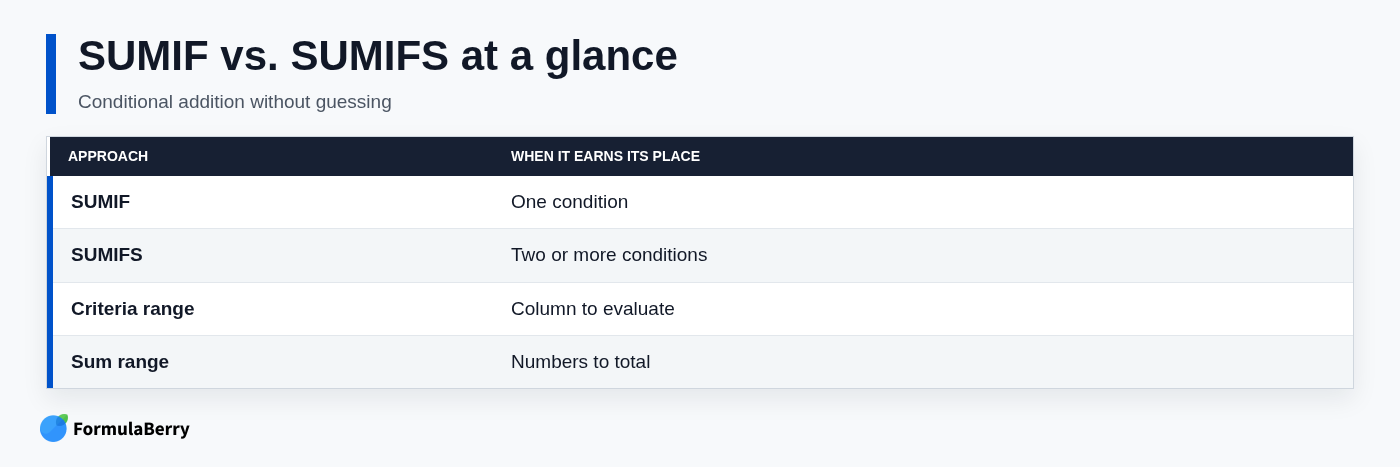
Conditional totals answer questions such as "How much has been paid?" or "What were East region sales this quarter?" Use SUMIF when there is one rule.

Suppose A2:A20 contains payment statuses and B2:B20 contains amounts. To add only rows marked Paid, use:

=SUMIF(A2:A20,"Paid",B2:B20)

The first range is the criteria range, or the cells Google Sheets checks. The word "Paid" is the criterion. The final range is the sum range, containing the amounts to total.

Use cell references instead of hard-coded criteria when you want a reusable report. For example, if E1 contains a status selected by the user, use =SUMIF(A2:A20,E1,B2:B20).

Use SUMIFS for multiple conditions

Use SUMIFS when every included row must meet two or more conditions. For example, this formula totals amounts in C2:C20 for the East region from January 1, 2026 onward:

=SUMIFS(C2:C20,A2:A20,"East",B2:B20,">="&DATE(2026,1,1))

Unlike SUMIF, SUMIFS puts the sum range first. After that, add each criteria range and criterion as a pair:

• C2:C20: values to add
• A2:A20, "East": include only East rows
• B2:B20, ">="&DATE(2026,1,1): include only rows on or after the specified date

For a report that changes by region or date, replace the fixed text and date with cell references. That lets one formula respond to filters or report controls without being rewritten.

Add totals from another sheet

To total values from another tab in the same workbook, include the sheet name followed by an exclamation mark. For example, to total January values in B2 through B31, use:

=SUM(January!B2:B31)

To add values from more than one monthly tab, list each range separately:

=SUM(January!B2:B31,February!B2:B28)

If a sheet name includes spaces, put it in apostrophes. A sheet called January Sales needs this syntax:

=SUM('January Sales'!B2:B31)

Google Sheets does not support Excel-style 3D references such as Sheet1:Sheet4!A2. List each sheet and range explicitly, or consolidate the monthly data into one table before calculating totals.

Avoid common cross-sheet reference errors

Start by testing one reference, such as =January!B2, before building a larger formula. If that works, expand it into a SUM formula.

The most common problems are a misspelled tab name, missing apostrophes around a name with spaces, and ranges that do not match across tabs. For example, make sure each monthly tab uses the intended amount column before adding them together.

Fix common errors when adding in Google Sheets

If your total is wrong or a formula produces an error, check the formula before rebuilding the sheet. A few issues account for most Google Sheets adding formula problems.

• #VALUE! often appears when a formula directly adds incompatible text, such as =A2+B2 where one referenced cell contains text. Check the inputs and confirm each reference is valid.
• #REF! means a formula refers to a cell, range, or sheet that no longer exists or was moved in a way Sheets cannot resolve. Restore or replace the broken reference.
• Unexpected zero totals can occur when values that look like numbers are stored as text. Reformat or convert those cells to numbers before summing.

Remember that SUM usually ignores text inside a selected range, while the plus sign can return an error when it directly encounters text. If a total seems too low, look for numeric-looking values that are actually text entries, often caused by copied data, leading apostrophes, or inconsistent imports.

Use this quick checking sequence: inspect the formula bar, confirm the range starts and ends in the correct cells, make sure you have not included another total, and verify that the input cells contain real numbers.

Prevent double-counting in a grand total

Do not sum a range that already includes subtotals. If rows 2 through 20 contain transaction details and row 21 contains a subtotal, a grand total should not use a range that includes both the detail rows and row 21 unless that is intentional.

Also avoid including the total cell itself, which can create a circular reference. Keep detail rows separate from summary rows, then point your total formula only at the detail range.

Use the formula that keeps your sheet easy to update

Use + for a few specific cells, SUM for a continuous range, and SUMIF or SUMIFS when rules determine which values belong in the total. Add the sheet name before a range whenever the numbers live on another tab.

If you know the calculation you need but not the exact Excel or Google Sheets formula, FormulaBerry can turn a plain-English request into a formula, explain an existing one, or help correct a formula that is not working.