The fastest way to filter out blank rows in Google Sheets is to use FILTER with a nonblank test on a reliable column: =FILTER(A2:D100,A2:A100<>""). It returns only the rows where column A contains a value, creating a clean version of your table that updates automatically when data changes within the referenced range.

This formula does not delete empty rows from the original data. Instead, it builds a separate output that changes automatically when records within rows 2 through 100 are added, removed, or filled in.

The simplest formula to filter out blank rows in Google Sheets

For a table in columns A through D where column A always contains an ID, date, name, or other required value, use:

=FILTER(A2:D100,A2:A100<>"")

The formula returns rows 2 through 100 from columns A through D, but only when the matching cell in column A is not empty. If a row has no value in A, it stays out of the filtered result.

This is usually the best answer to "how can I filter out empty rows in Google Sheets?" because it preserves the source data and gives you a live report range elsewhere in the workbook.

How Google Sheets FILTER handles nonblank rows

FILTER has two essential parts: the data you want returned and the condition that decides which rows qualify. In =FILTER(A2:D100,A2:A100<>""), A2:D100 is the output range and A2:A100<>"" is the condition.

The <>"" portion means "is not equal to an empty string." Google Sheets checks each cell in A2:A100 and keeps the corresponding row only when that test is true.

The condition range must cover the same number of rows as the range you are filtering. For example, filtering A2:D100 with a condition based on A2:A99 causes a range-size error because one range has 99 rows and the other has 98.

Once entered, the output updates on its own when data changes within the referenced range. Add a new value to the source table between rows 2 and 100, and the filtered view changes without sorting, copying, or reapplying a filter.

Choose the column that defines whether a row is blank

Use a column that should be filled for every legitimate record. Good choices include an invoice number, customer email, transaction date, product name, or employee ID.

Do not automatically use the first column just because it is column A. If A contains optional notes while the rest of the row contains useful data, the formula will exclude valid records whenever that notes cell is empty.

For example, a sales table may have optional comments in column A and required order IDs in column B. In that case, test column B instead:

=FILTER(A2:D100,B2:B100<>"")

Copy-paste formulas for common blank-row scenarios

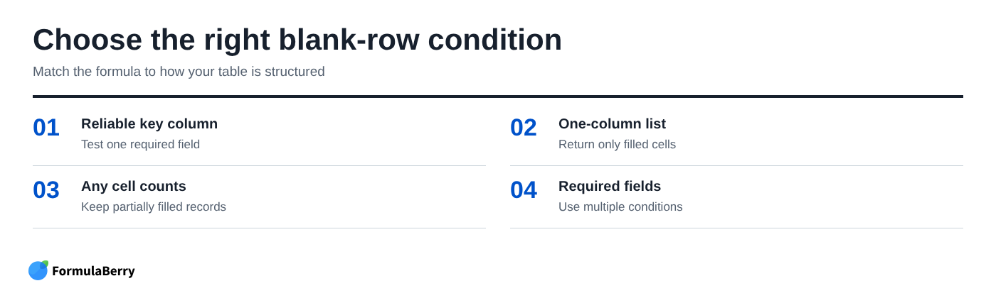
The right formula depends on how your sheet is structured. A table with a dependable ID column needs a simpler condition than a loosely filled intake sheet where any cell may contain data.

These examples use bounded ranges, which are usually easier on large workbooks than full-column references such as A:A. Whole-column formulas are convenient for smaller sheets, but they can make a busy workbook recalculate more slowly.

Filter rows where column A is not blank

Use this when column A is the dependable identifier for each record:

=FILTER(A2:D100,A2:A100<>"")

It returns a four-column table and skips every row with an empty value in column A. This is the standard filter-if-not-blank Google Sheets formula for a structured table.

Filter a single column and remove empty cells

If you only need a cleaned list from one column, use:

=FILTER(A2:A100,A2:A100<>"")

This is useful for creating a dropdown source list, a compact list of email addresses, or a list of item names. Unlike a multi-column FILTER, it does not preserve related fields from the same records because it only returns values from column A.

Keep rows when any cell in the row contains data

When no single column is consistently filled, test the entire row instead:

=FILTER(A2:D100,BYROW(A2:D100,LAMBDA(row,COUNTA(row)>0)))

This keeps a row if at least one cell in columns A through D contains data. It is useful for partially completed forms, rough imports, or shared sheets where people enter details in different columns.

Check that your Google Sheets environment supports BYROW and LAMBDA before relying on this approach. If your sheet does not support them, a helper column is often the clearest fallback. For formulas that apply the same calculation across a range, see this guide to Array Formula in Google Sheets.

Keep rows only when every required field is filled

To return records only when both column A and column B contain values, use:

=FILTER(A2:D100,(A2:A100<>"")*(B2:B100<>""))

The asterisk works as AND logic here. A row is returned only if the test for column A and the test for column B are both true.

Add more conditions when needed. For example, a contact list may require a name, email address, and signup date before it belongs in a reporting view.

Why FILTER can still return rows that look blank

A row can look empty to you but not be truly empty to Google Sheets. The usual causes are formulas that return empty strings, ordinary spaces, copied nonbreaking spaces, and other hidden characters.

This matters because an unused cell, a cell containing a formula, and a cell containing a space are different things. In particular, ISBLANK can give surprising results when a cell contains a formula that displays nothing.

Cells containing formulas that return an empty string

A formula such as =IF(C2="","",C2*10) may display a blank result, but the cell still contains a formula. That is why testing for physical emptiness with ISBLANK is often the wrong choice for cleanup formulas.

If you want to keep only visibly populated values, test the text length instead:

=FILTER(A2:D100,LEN(A2:A100)>0)

This condition excludes cells whose displayed result is an empty string. Use it when your key column contains formulas that intentionally return "" when there is nothing to show.

Spaces and hidden characters

A cell containing one or more spaces passes the test A2:A100<>"", even though it may look blank. For normal stray spaces, trim the text before testing it:

=FILTER(A2:D100,LEN(TRIM(A2:A100))>0)

This is especially useful after copying data from forms, emails, or other spreadsheets. If the source contains nonbreaking spaces or unusual imported characters, TRIM may not be enough. Depending on the source, you may need to remove a specific character with SUBSTITUTE or clean the text with CLEAN before applying the length test.

FILTER versus deleting or hiding empty rows

Filtering out empty rows, hiding them, and deleting them are three different tasks. Choose the method based on whether you need a report, a temporary view, or a permanent cleanup.

• Use FILTER when you want a separate, live output for a dashboard, report, export area, or summary tab.
• Use Google Sheets filter views when you want to browse nonblank records in the original table without changing the underlying data.
• Delete rows only when those rows are genuinely unwanted and you are comfortable making a permanent source-data change.

For most reporting work, FILTER is safer than deleting rows. It leaves the original table intact and prevents new blank gaps from breaking a carefully prepared report later.

Avoid common FILTER errors

Most FILTER problems come from range mismatches or blocked output cells, not from the nonblank condition itself. A few checks solve the majority of issues.

• Range sizes do not match: Make sure the returned range and every condition range start and end on matching rows. If you filter A2:D100, use conditions that also run from row 2 through row 100.
• The result cannot expand: FILTER returns multiple rows and columns. Clear any values, formulas, or merged cells in the destination area below and to the right of the formula.
• No matching rows: If nothing meets the condition, Sheets returns a no-results error. That is accurate, but it may not be the message you want in a report.

To show a friendlier message when no rows qualify, wrap the formula in IFNA:

=IFNA(FILTER(A2:D100,A2:A100<>""),"No matching rows")

Use IFNA deliberately. It is helpful for a finished report, but while building a formula, the original error can make it easier to spot a bad range or condition.

Build a clean, self-updating Google Sheets view

Start with the simplest rule that matches your data: test one reliable key column when every valid record has one. Use a whole-row test only when a row can be valid with data in different places, and add multiple conditions when a record must include specific required fields.

A dynamic FILTER output is usually a better solution than trying to repeatedly remove empty rows from a changing source range. It keeps reports tidy while preserving the original data for review and correction.

If you need to adapt a FILTER condition for your own columns or combine it with other Google Sheets logic, FormulaBerry can generate, explain, or help correct the formula from a plain-language description of your sheet.