

Spreadsheet data rarely arrives in the shape you need. Names may be spread across several columns, tags may sit in a row, and a report may contain empty cells or errors that make a simple list difficult to create.
The Excel TOCOL function solves that problem by turning a range into one dynamic, vertical list. Once you understand its scan order and ignore settings, it becomes a practical tool for cleaning lists, preparing data for validation dropdowns, and consolidating values without manually copying cells.
What the TOCOL function does in Excel
TOCOL means "to column." It is a dynamic-array function that takes a range or array and returns every value in a single spilled column.
For example, if values occupy several rows and columns, TOCOL can stack them into one clean vertical list. This is useful when you need a source list for a report, a dropdown, a lookup table, or a duplicate check.
TOCOL does not alter the original cells. Instead, you enter one formula in a destination cell, and Excel creates a new spill range below it. If the original range changes, the returned list updates automatically.
Check that your Excel version supports TOCOL
TOCOL is available in modern Microsoft 365 versions of Excel and Excel for the web, where dynamic-array functions are supported. If Excel displays #NAME? after you enter TOCOL, your installed version probably does not include the function.
To check your version in the desktop app, go to File > Account > About Excel. Microsoft 365 subscribers should also make sure Office updates are installed. Excel for the web is often the quickest way to confirm whether the function is available in your account.
Older perpetual versions of Excel, such as many installations of Excel 2019 or earlier, may not recognize TOCOL. You can still reshape data with alternatives such as TRANSPOSE, Power Query, or a one-time paste operation, covered later in this guide.
Learn the TOCOL syntax and its three arguments
The full syntax is:
=TOCOL(array, [ignore], [scan_by_column])
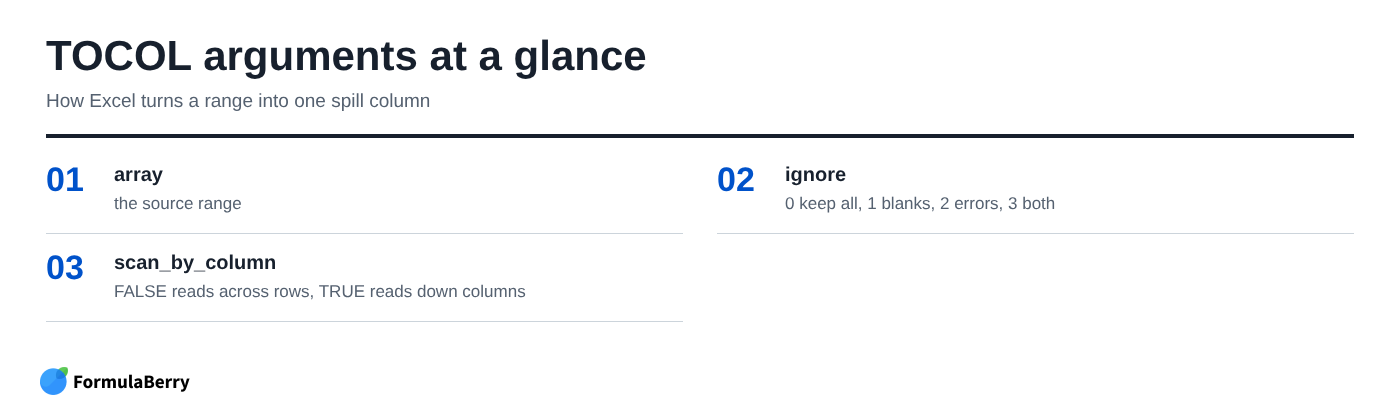
Only the first argument is required. The other two arguments control which values Excel includes and the order in which it reads the range.
- array: The source range or array to turn into one column, such as A2:C20.
- ignore: An optional number that tells Excel whether to omit blank cells and errors.
- scan_by_column: An optional TRUE or FALSE setting that controls whether Excel reads across rows or down columns.
The ignore argument accepts four values:
- 0: Keep blanks and errors. This is the default.
- 1: Ignore blank cells.
- 2: Ignore error values.
- 3: Ignore both blanks and errors.
By default, TOCOL scans across each row before moving to the next row. For a range such as A2:C4, Excel reads A2, B2, C2, then A3, B3, C3, and so on. Set the third argument to TRUE when you want Excel to read down the first column before moving to the next one.
Convert a simple range to one column with the basic TOCOL formula
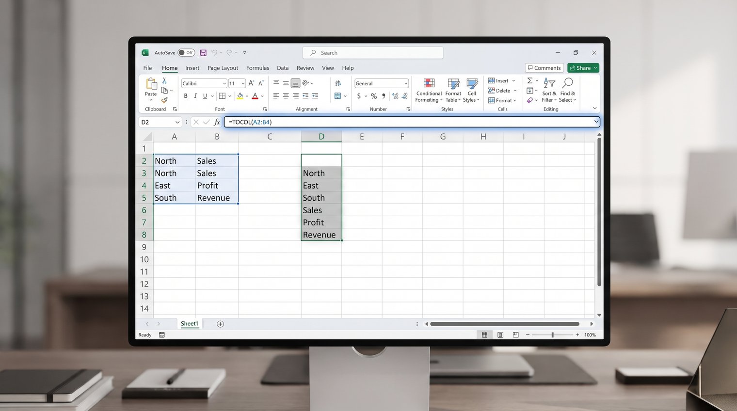
Start with a small rectangular range. If your source data is in A2:C4, click an empty cell with enough open space below it and enter:
=TOCOL(A2:C4)
Suppose the source contains these values:
| A | B | C |
|---|---|---|
| Red | Blue | Green |
| Orange | Purple | Yellow |
| Black | White | Gray |
The formula returns Red, Blue, Green, Orange, Purple, Yellow, Black, White, and Gray in one vertical column. Excel reads left to right across the first row, then continues with the next row.
Enter the formula once and press Enter. Do not drag it down. TOCOL is a dynamic-array formula, so Excel spills the result into the required number of cells automatically.
Common mistake: entering the formula beside data that extends below the formula cell. If any cell in the planned spill range contains a value, Excel returns #SPILL!. Move the formula or clear only the cells that are genuinely blocking the result.
Choose the right scan order for your data
The default formula, =TOCOL(A2:C4), uses row-first scanning. With the sample range above, that produces Red, Blue, Green, Orange, Purple, Yellow, Black, White, and Gray.
To read down each column first, use:
=TOCOL(A2:C4,,TRUE)
Notice the two commas. The second argument is being left at its default value, while TRUE is supplied for the third argument. This version returns Red, Orange, Black, Blue, Purple, White, Green, Yellow, and Gray.
Use row-first order when each row represents a record and its values should remain together in sequence. Use column-first order when each column is a separate vertical list that you want to append one after another.
Changing scan order does not change the underlying values. It only changes the sequence in the resulting list, which matters when you plan to match positions, review entries in order, or feed the list into another formula.
Ignore blanks, errors, and unwanted zero values
In real workbooks, blank cells are usually the first obstacle. To combine a range into a compact list without empty positions, use:
=TOCOL(A2:C20,1)
The 1 instructs Excel to ignore blank cells. If the range can also contain formula errors such as #N/A or #DIV/0!, use:
=TOCOL(A2:C20,3)
This ignores both blanks and error values. Use it carefully: excluding an error may be appropriate for a display list, but it can also conceal a source-data problem that needs attention.
Zero is different from a blank. TOCOL treats 0 as a legitimate value, so =TOCOL(A2:C20,1) will keep zeroes. If you need a list that excludes blanks and zeroes, filter first and then stack the remaining cells:
=TOCOL(FILTER(A2:C20,(A2:C20<>"")*(A2:C20<>0)),1)
FILTER removes cells that are blank or equal to zero. TOCOL then converts the filtered result into one vertical spill range. The final ,1 is a sensible safeguard if the filtered result can still include blank cells.
Keep only values that meet multiple conditions
For a TOCOL Excel formula with multiple criteria, apply the criteria with FILTER before using TOCOL. Imagine a sales table where column A contains product names, column B contains regions, and column C contains sales amounts. To create a list of products sold in the West region with sales above 1,000, use:
=TOCOL(FILTER(A2:A20,(B2:B20="West")*(C2:C20>1000)),1)
Each condition is wrapped in parentheses, and the asterisk works as AND logic. FILTER returns only the product names whose aligned region and sales cells satisfy both conditions. TOCOL then ensures the result is a clean single column.
Criteria ranges must align with the array being filtered. If you filter A2:A20, use criteria ranges that also run from row 2 through row 20. When filtering a rectangular range such as A2:C20, each condition still needs one result per source row.
Flip one row into one column
If your data occupies one horizontal row, TOCOL provides a quick row-to-column conversion. For values in A1:F1, enter:
=TOCOL(A1:F1)
The values spill downward in the same left-to-right order. For a partially filled row where unused cells should not appear in the result, use:
=TOCOL(A1:F1,1)
For a simple orientation flip, =TRANSPOSE(A1:F1) is also a straightforward choice. TRANSPOSE is especially clear when your only goal is to turn a known row into a column.
TOCOL becomes more useful when the selected range may later grow into multiple rows or columns, or when you want to ignore blanks and control scan order at the same time.
Combine several adjacent columns into one clean list
A common use case is consolidating entries spread across neighboring columns. For example, a worksheet may store product tags in A2:C10, with one, two, or three tags assigned to each product.
To turn those columns into one compact list, use:
=TOCOL(A2:C10,1)
Excel reads across each row by default and skips blank cells. The output remains live: add a tag to the selected source range and it appears in the spilled list.
TOCOL stacks values, but it does not remove repeated items. If "Seasonal" appears in five source cells, it will appear five times in the result. That is correct when frequency matters, but it is not the same as creating a unique list.
Build more useful lists with TOCOL and other functions
TOCOL is most useful when it is the first or middle step in a focused formula. Add other functions only when the final list needs a specific treatment.
To create a distinct list from a range containing duplicates and blanks, use:
=UNIQUE(TOCOL(A2:C20,1))
TOCOL creates the clean vertical list, while UNIQUE keeps only the first occurrence of each value. If you also want the result in alphabetical or numerical order, wrap it in SORT:
=SORT(UNIQUE(TOCOL(A2:C20,1)))
Text cleanup should usually happen before stacking. If imported data includes unwanted leading or trailing spaces, use:
=TOCOL(TRIM(A2:C20),1)
TRIM removes extra spaces from each text value, and TOCOL returns the cleaned entries in a single column. This matters because "North" and "North " look identical in a worksheet but are treated as different values by functions such as UNIQUE.

Fix common TOCOL errors and spill problems
A #NAME? error usually means your Excel version does not support TOCOL or Excel does not recognize the function name. Confirm your version before rebuilding the formula. Changing commas to semicolons may be necessary in some regional Excel settings, but it will not solve a missing function.
A #SPILL! error means the output range is blocked. Select the formula cell and use Excel's error indicator to identify the obstruction. Then clear, move, or relocate only the cells preventing the spill result. Also check whether the formula is inside an Excel Table, since spilled array formulas cannot spill within table columns.
If the list contains unexpected values, first inspect the selected array. It is easy to include an extra header row, an unused column, or a range with hidden formula results. Then check whether the issue is caused by the ignore argument or the scan order.
When building a more complex formula, test TOCOL on a small range first. Confirm that the output order is right before adding FILTER, UNIQUE, SORT, or other functions around it.
Why the result includes blank rows or error values
If your output includes blanks, replace the default formula with =TOCOL(A2:C20,1). If it includes errors you intentionally want to omit, use =TOCOL(A2:C20,2), or =TOCOL(A2:C20,3) to exclude both errors and blanks.
Do not assume every empty-looking cell is truly blank. A formula that returns an empty text string, written as "", can behave differently from a cell that contains nothing at all. If the result surprises you, inspect the source formulas and test a few cells individually before deciding which ignore setting to use.
Use a TOCOL alternative when the function is unavailable
The best TOCOL function alternative depends on whether you need a live, updating output or a one-time conversion.
For flipping one row into one column, use TRANSPOSE. It is widely understood and works well when the source is a straightforward single row or single column.
For repeatable reshaping of larger imported datasets, use Power Query. It is a better fit when you regularly need to unpivot columns, remove blanks, clean imported values, and refresh the result from the same source structure.
For a one-off static conversion, copy the source range, select a destination cell, and use Paste Special > Transpose if you only need to switch rows and columns. This creates values rather than a live connection, so later edits to the source will not update the pasted result.
Older INDEX-based formulas can sometimes mimic parts of TOCOL, but they are harder to maintain and rarely worth the effort for ordinary spreadsheet work. If your workbook needs a live, flexible list and TOCOL is unavailable, Power Query is generally the more reliable route.
Turn ranges into reliable single-column lists
TOCOL is simple once you make four decisions: select the right source array, choose whether to ignore blanks or errors, confirm the scan direction, and add FILTER, UNIQUE, or SORT only when the final list requires it.
Start with the basic pattern =TOCOL(range,1) for most clean-list tasks. Then adjust scan order or filter criteria when the source layout calls for it. Keeping the formula focused makes it easier to audit when the workbook changes.
If you can describe the spreadsheet result you need but are unsure how to write the formula, FormulaBerry can generate, explain, and help correct Excel and Google Sheets formulas from a plain-language request.