A COUNTIF formula looks simple until the criterion gets even slightly more specific. Counting "Paid" is easy; counting values above a changing target, orders containing a word, or dates within a month is where misplaced quotes and date formats start producing the wrong result.

This guide shows how to use COUNTIF in Google Sheets for text, numbers, dates, cell references, and duplicate checks. You will also see when COUNTIFS is the better choice.

COUNTIF syntax: the one-condition counting formula

The basic Google Sheets COUNTIF formula is:

=COUNTIF(range, criterion)

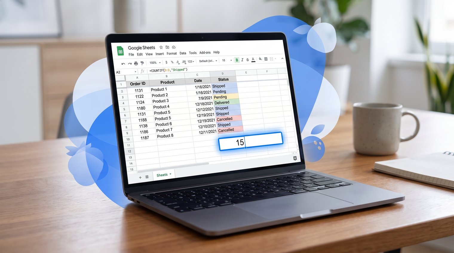
COUNTIF returns the number of cells in one range that meet one condition. The range is where Google Sheets should look, and the criterion is what each cell must match.

Column A: Order status	Example formula	Result
Paid	=COUNTIF(A2:A6,"Paid")	3
Pending
Paid
Refunded
Paid

In this example, A2:A6 is the range and "Paid" is the criterion. Text criteria need quotation marks. Numeric criteria often do not, unless you are combining a number with an operator such as greater than or equal to.

FormulaBerry

If you know what you need to count but cannot remember the exact syntax, FormulaBerry can turn a plain-English request into a Google Sheets or Excel formula. For example, you could ask for a formula that counts orders marked Paid, or counts invoice amounts above a target stored in another cell.

It is especially useful when the criterion includes operators, dates, or multiple conditions that are easy to mistype. It does not replace the need to verify your selected columns and ranges, so always confirm that the generated formula points to the correct cells in your sheet.

How criteria work: text, numbers, operators, and cell references

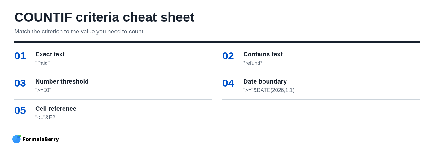
The criterion changes depending on the value you want to count. Use quoted text for a label, quote comparison operators, and join an operator to a cell reference with an ampersand.

• =COUNTIF(A2:A100,"Paid") counts exact text matches.
• =COUNTIF(B2:B100,">=50") counts values equal to or greater than 50.
• =COUNTIF(C2:C100,"<="&E2) counts values less than or equal to the value in E2.

The ampersand combines pieces of a criterion. In the last example, Google Sheets builds a criterion such as <=100 when E2 contains 100. Writing <=E2 inside quotation marks will not work because Sheets treats E2 as text rather than as a cell reference.

Count text values and cells that contain specific text

Text-based COUNTIF formulas are useful for order statuses, task stages, categories, customer comments, and simple dashboard summaries. Start with an exact match when your labels are standardized. Use wildcards when the text may appear as part of a longer entry.

Exact text, partial text, and wildcard examples

To count an exact status label, use:

=COUNTIF(A2:A100,"Complete")

This counts cells whose value is Complete. For cells that contain the word refund anywhere in the text, use asterisks as wildcards:

=COUNTIF(A2:A100,"*refund*")

The asterisk means "any number of characters." It would match Refund requested, partial refund, and refund processed. COUNTIF is case-insensitive, so Refund and refund are treated the same.

To count cells containing text, use:

=COUNTIF(A2:A100,"*")

To count all nonempty cells, including numbers, use:

=COUNTA(A2:A100)

To count blank cells, use:

=COUNTIF(A2:A100,"")

Be careful with apparent blanks. A cell containing a space is not empty, even though it may look empty on screen. If someone pasted values from another system, hidden spaces can make blank counts and text matches unreliable.

The question mark wildcard matches exactly one character. For example, =COUNTIF(A2:A100,"Item-?") matches Item-A and Item-7, but not Item-AB. If you need to find a literal asterisk or question mark, put a tilde before it: use "~*" for an asterisk and "~?" for a question mark.

Count numbers, values above or below a threshold, and numbers in a range

For an exact number, COUNTIF is straightforward:

=COUNTIF(B2:B100,25)

That counts cells containing the number 25. For comparisons, place the operator and value together inside quotation marks:

• =COUNTIF(B2:B100,">50") counts values above 50.
• =COUNTIF(B2:B100,"<=100") counts values of 100 or less.
• =COUNTIF(B2:B100,"<>0") counts values that are not zero.

COUNTIF does not calculate arithmetic expressions inside its criterion. For example, =COUNTIF(B2:B100,">50+10") does not mean greater than 60. Calculate the threshold in a cell first, then reference that cell, or write the final value directly.

Count values between two numbers

To count values from 10 through 25, including both endpoints, use COUNTIFS:

=COUNTIFS(B2:B100,">=10",B2:B100,"<=25")

Although the same column appears twice, this is still a multiple-condition formula: each value must be at least 10 and no more than 25. To exclude the endpoints, replace >= and <= with > and <.

You can add separate COUNTIF results, but COUNTIFS is cleaner and safer for a between-two-numbers condition. It ensures both tests apply to the same cell.

Count dates correctly in Google Sheets

Google Sheets stores dates as serial numbers, which is why the same comparison pattern used for numbers also works for dates. The reliable approach is to use DATE() rather than typing a date as text, because typed date formats can be interpreted differently depending on spreadsheet locale.

For dates before January 1, 2026:

=COUNTIF(A2:A100,"<"&DATE(2026,1,1))

For dates on or after January 1, 2026:

=COUNTIF(A2:A100,">="&DATE(2026,1,1))

A common mistake is using an inclusive end date when the column contains timestamps. A value such as January 31, 2026 at 3:00 PM is later than the serial value for January 31 at midnight, so it may be missed by an end-date test using <=DATE(2026,1,31).

Count dates in a month or date range

For all dates in January 2026, use the first day of the month as the lower boundary and the first day of the next month as an exclusive upper boundary:

=COUNTIFS(A2:A100,">="&DATE(2026,1,1),A2:A100,"<"&DATE(2026,2,1))

This formula includes every January date and timestamp without needing to know whether the month has 28, 30, or 31 days. The same pattern works for reporting periods, billing cycles, and weekly date windows.

Use a cell reference as the COUNTIF criterion

Hard-coding a status or threshold is fine for a quick calculation, but a cell reference makes a formula reusable. This is the better choice for a dashboard, report template, or sheet someone else will update.

Suppose F2 contains the status you want to count. Use:

=COUNTIF(A2:A100,F2)

Change F2 from Paid to Pending, and the count updates automatically. For numeric comparisons, join the operator to the reference:

=COUNTIF(B2:B100,">="&F2)

If you plan to copy the formula across or down, use an absolute reference when the input cell should remain fixed:

=COUNTIF($A$2:$A$100,$F$2)

For a dynamic status summary, place status labels in D2:D5 and enter =COUNTIF($A$2:$A$100,D2) in E2. Copy it down beside each label. This avoids maintaining a separate formula for Paid, Pending, Complete, and every other status. For more advanced range-based calculations, see this guide to an array formula in Google Sheets.

Find duplicates with COUNTIF

COUNTIF is one of the quickest ways to identify duplicate invoice numbers, email addresses, product codes, or customer IDs. The right formula depends on whether you want to flag only later repeats or every value that occurs more than once.

To identify a duplicate starting with the second occurrence, use:

=COUNTIF($A$2:$A2,A2)>1

Enter it in row 2 beside your data and copy it down. The first part of the range, $A$2, stays fixed. The second part, $A2, expands as the formula moves down. The first instance returns FALSE; later occurrences return TRUE.

To flag every repeated value, including the first occurrence, use:

=COUNTIF($A$2:$A$100,A2)>1

This checks the full list each time. You can use the same logic in a conditional formatting custom formula to highlight duplicate records.

Flag duplicates without flagging blank rows

Blank cells are often repeated many times, so a basic duplicate rule can highlight every empty row. Exclude blanks with:

=AND(A2<>"",COUNTIF($A$2:$A$100,A2)>1)

Adjust A2 and the ending row to match your actual identifier column and starting row. If your IDs are in column C and data starts in row 5, the references should use C5 instead.

When to use COUNTIFS instead of COUNTIF

Use COUNTIF for one condition in one range. Use COUNTIFS when a row must meet two or more conditions. COUNTIFS takes range-and-criterion pairs, and every condition must be true for the row to be counted.

All COUNTIFS ranges must cover the same dimensions. If one range is A2:A100 and another is B2:B99, the formula will fail or return an unreliable result.

Count rows that meet two conditions

To count tasks assigned to the West region that are also marked Complete, use:

=COUNTIFS(A2:A100,"West",B2:B100,"Complete")

The first pair checks column A for West. The second pair checks column B for Complete. Only rows meeting both tests are counted.

COUNTIF cannot evaluate these two separate column conditions by itself. Do not try to force both conditions into one text criterion; move to COUNTIFS instead.

Add a third criterion or a date window

COUNTIFS can take additional pairs when you need a more specific report. For example, to count completed West-region tasks assigned to Jordan:

=COUNTIFS(A2:A100,"West",B2:B100,"Complete",C2:C100,"Jordan")

For completed tasks due in January 2026, include the date range as two additional conditions:

=COUNTIFS(B2:B100,"Complete",D2:D100,">="&DATE(2026,1,1),D2:D100,"<"&DATE(2026,2,1))

Keep formulas readable by using one clear range/criterion pair at a time. If you find yourself stacking unrelated logic into one formula, a helper column may be easier for the next person to understand.

Count across multiple ranges without double-counting

COUNTIF accepts one range at a time. If you need to total matches in separate, non-overlapping ranges, add individual COUNTIF results:

=COUNTIF(A2:A20,"Yes")+COUNTIF(C2:C20,"Yes")

This is appropriate when columns A and C are separate lists. It is not the same as checking whether two conditions occur on the same row. For same-row conditions across columns, use COUNTIFS. If you need more examples of adding values and ranges, see the Excel SUM formula guide.

Be cautious when combining ranges from different sections of a sheet. If the same record can appear in both ranges, adding counts will count it twice. A helper column is often the safest default for complex logic: mark qualifying records once, then count the helper-column results.

COUNT vs. COUNTIF: choose the right function

COUNTIF is not always the right counting function. Choose based on what you actually need to measure:

• COUNT counts cells containing numbers only.
• COUNTA counts cells that are not empty.
• COUNTBLANK counts blank cells.
• COUNTIF counts cells that match one specified condition.

The practical rule is simple: if you only need the number of numeric entries, use COUNT. If you need to count a particular value, text label, threshold, or pattern, use COUNTIF. If your calculation requires several tests, use COUNTIFS.

Fix common COUNTIF errors and unexpected results

When COUNTIF returns zero or a number that feels wrong, the problem is usually in the underlying cell values or criterion format rather than the function itself.

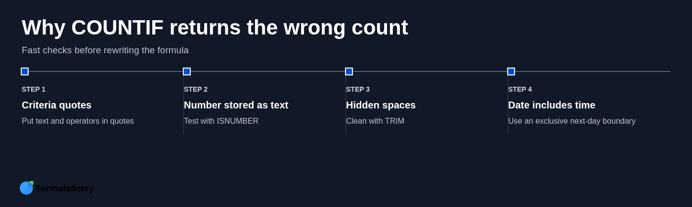
• Text numbers: A value that looks like 50 may be stored as text. Test a cell with =ISNUMBER(B2). Formatting a cell as a number does not always convert its stored value.
• Hidden spaces: A status such as "Paid " will not reliably match "Paid". Check the length with =LEN(A2) and clean imported text with =TRIM(A2).
• Incorrect quotes: Text and comparison operators need quotation marks. Use ">=50", not >=50.
• Missing concatenation: For an operator based on a cell value, use ">="&F2, not ">=F2".
• Date and time mismatches: Use a next-day or next-month exclusive upper boundary when timestamps are present.

COUNTIF is case-insensitive. It treats paid, Paid, and PAID as matches. If case sensitivity is essential, use an advanced approach based on SUMPRODUCT and EXACT rather than trying to force COUNTIF to distinguish capitalization.

Build reliable Google Sheets counts from clear criteria

Start with COUNTIF when you have one condition: a status, a text pattern, a numeric threshold, or a date boundary. Use cell references when the criterion needs to change, and move to COUNTIFS as soon as multiple conditions must be true on the same row.

The most reliable formulas use clean source data, correctly quoted operators, and date windows built with DATE(). If you can describe the count you need in plain language but are unsure how to write it, the Excel formula generator can generate, explain, or help correct the appropriate Excel or Google Sheets formula.