Excel does not have a standalone CONTAINS function, which is why a simple request such as "check whether this cell includes apple" can turn into a confusing formula hunt. The reliable approach is to use SEARCH or FIND inside ISNUMBER, then add IF or FILTER when you need a useful result rather than just TRUE or FALSE.

This guide covers the Excel contains formula patterns that matter in everyday worksheets: partial text, case-sensitive matches, multiple terms, and returning values from matching rows. These formulas test whether a cell contains text. They do not test whether a cell contains an Excel formula.

Choose the right way to test whether Excel contains text

There is no CONTAINS function in Excel. For most cases, use SEARCH inside ISNUMBER:

=ISNUMBER(SEARCH("text",A2))

SEARCH looks for text inside A2. If it finds the text, it returns a number representing the starting position. If it cannot find the text, it returns an error. ISNUMBER converts those outcomes into the more useful TRUE or FALSE result.

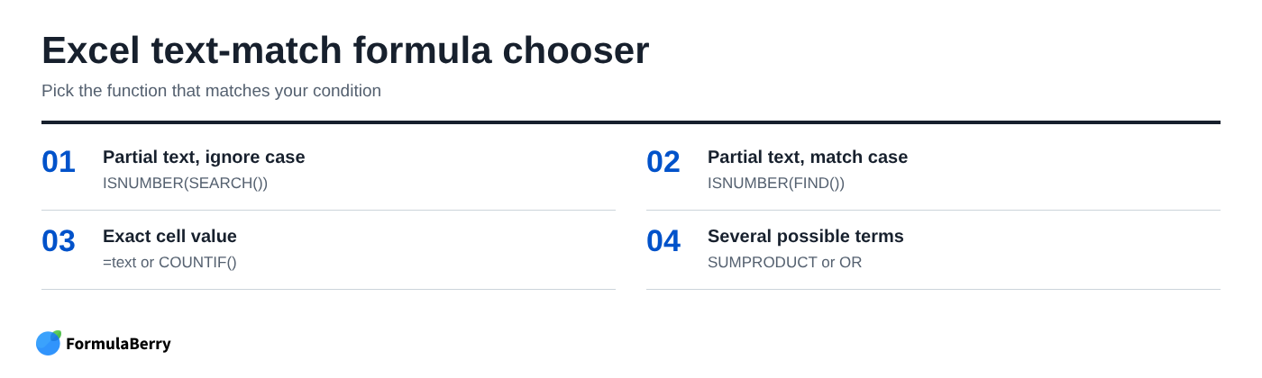
• Partial text, ignore case: =ISNUMBER(SEARCH("apple",A2))
• Partial text, match case: =ISNUMBER(FIND("Apple",A2))
• Exact cell value: =A2="apple"
• Exact match anywhere in a range: use COUNTIF or a direct comparison
• Several possible terms: use OR for a few terms or a criteria list for more scalable matching

Use SEARCH when capitalization does not matter. Use FIND when it does. If the full cell must equal a specific value, do not use a contains formula at all; use an exact comparison instead.

Test whether a cell contains specific text with SEARCH

The most common Excel formula if a cell contains specific text is:

=ISNUMBER(SEARCH("apple",A2))

This formula checks whether the contents of A2 include the text "apple." It returns TRUE for values such as "Green apple," "APPLE JUICE," and "Organic apples." It returns FALSE if A2 contains "Orange soda."

SEARCH has two relevant arguments here: the text you want to find and the cell to inspect. For example, =SEARCH("apple",A2) returns 7 if "apple" begins with the seventh character in A2. When the word is absent, SEARCH produces a #VALUE! error. Wrapping it in ISNUMBER prevents that error from appearing in your worksheet.

SEARCH is case-insensitive. "apple," "Apple," and "APPLE" all count as matches.

Return a custom result with IF

A TRUE or FALSE result is useful for filtering, but labels are often easier to read in a report. Wrap the test in IF:

=IF(ISNUMBER(SEARCH("apple",A2)),"Match","No match")

If A2 contains "apple," Excel returns Match. Otherwise, it returns No match. You can replace those labels with a category, status, numeric flag, or any other result your worksheet needs.

For example, a product list might use this formula to label apple-related items for a seasonal promotion. A budget worksheet could use the same pattern to flag transaction descriptions containing "travel."

Check for partial text, including words inside longer strings

SEARCH finds text anywhere in a cell, not only at the beginning or end. That is what makes it useful for partial-text matching in Excel.

For example, this formula returns TRUE if A2 contains the letters "pro":

=ISNUMBER(SEARCH("pro",A2))

It would match "Pro Keyboard," "professional camera," and "approved product." That flexibility is useful when product names or descriptions are inconsistent, but it can also create matches you did not intend.

If you are looking for a whole word rather than a fragment, make the condition more precise. A search for "pro" is usually too broad. A search for "pro " or " pro " may work when your source text follows a consistent format, but it will not catch every punctuation pattern or word at the beginning or end of a cell.

Avoid false matches when the text fragment is too broad

Short search terms are the most common source of bad contains-text results. Searching for "cat" can match "category," "catalog," and "vacation," not just the animal or product category you intended.

When the data is standardized, search for surrounding characters that establish a boundary. For a comma-separated tag field, for example, you could standardize entries as ",apple,pear," and search for ",apple," rather than "apple." For imported or inconsistent data, clean and normalize the text before relying on a whole-word rule.

Common mistake: assuming a partial-text formula understands word boundaries. SEARCH does not. It only looks for a sequence of characters.

Make the contains test case-sensitive with FIND

Use FIND instead of SEARCH when uppercase and lowercase letters carry meaning:

=ISNUMBER(FIND("Apple",A2))

Unlike SEARCH, FIND is case-sensitive. If A2 contains "Apple pie," the formula returns TRUE. If it contains "apple pie," the formula returns FALSE.

FIND still returns a character position when it succeeds and a #VALUE! error when it fails, so ISNUMBER is still necessary for a clean TRUE or FALSE result.

Case-sensitive matching is most useful for product codes, status labels, identifiers, and structured data where capitalization is deliberate. It is usually the wrong default for ordinary product descriptions, notes, customer comments, or imported text, where inconsistent capitalization is common.

Return matching values from another column

Finding a matching row is only half the task. Often, you need Excel to return a related value from another column.

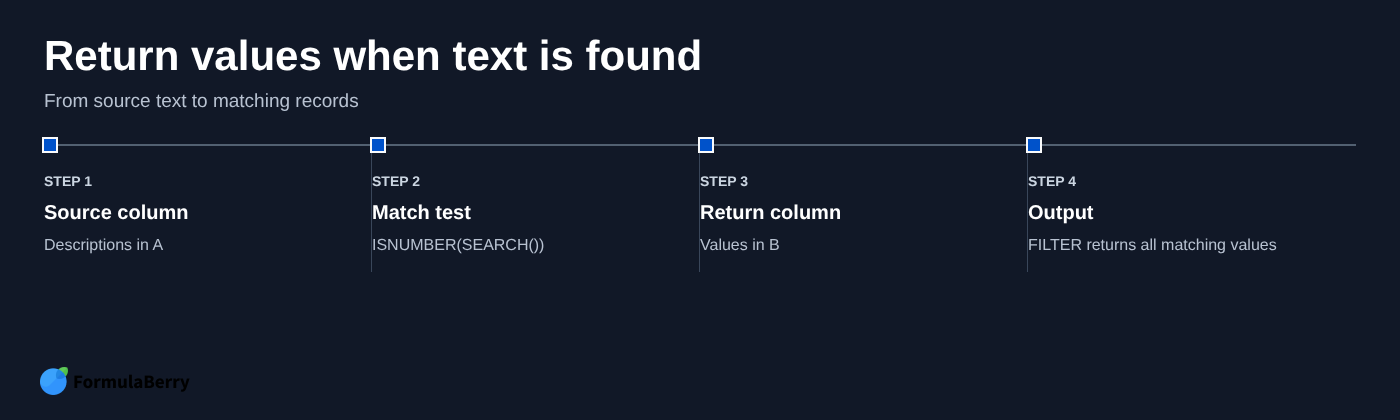
Suppose column A contains product descriptions and column B contains product IDs or prices. To return the value from B2 only when A2 contains "apple," use:

=IF(ISNUMBER(SEARCH("apple",A2)),B2,"")

If the description in A2 matches, Excel returns the corresponding value from B2. If not, it returns a blank cell. Copy the formula down to evaluate each row.

This helper-column method is practical when you want the original row structure to stay visible. You can filter out blanks later, or use a separate TRUE/FALSE helper column if you need to sort, filter, or audit the match condition independently.

Return all matching records with FILTER

In modern versions of Excel, FILTER can return every matching value in one formula:

=FILTER(B2:B100,ISNUMBER(SEARCH("apple",A2:A100)),"No matches")

Excel tests each description in A2:A100 for "apple." For every matching row, it returns the corresponding value from B2:B100. The results spill down automatically into adjacent cells.

Make sure the source and return ranges cover the same rows. If your descriptions are in A2:A100, the values you want to return must also run from row 2 through row 100.

Older Excel versions do not support FILTER. In that case, use the helper-column formula, then apply Excel's standard Filter to show only matching rows.

Test for any of several text values in one cell

Sometimes a cell can match any one of several terms. For a short, fixed list, OR is the clearest formula pattern:

=OR(ISNUMBER(SEARCH("red",A2)),ISNUMBER(SEARCH("blue",A2)))

This returns TRUE when A2 contains red, blue, or both. It returns FALSE only when neither term appears.

To return a label rather than TRUE or FALSE, wrap it in IF:

=IF(OR(ISNUMBER(SEARCH("red",A2)),ISNUMBER(SEARCH("blue",A2))),"Color match","")

Use this approach for two or three stable conditions. Once the list gets longer, maintaining a chain of SEARCH functions becomes error-prone.

Search a list of terms instead of hard-coding each one

Put the allowed terms in a small range, such as E2:E5, then test that list against the text in A2:

=SUM(--ISNUMBER(SEARCH(E2:E5,A2)))>0

The formula checks every term in E2:E5 and counts how many are found in A2. If one or more terms match, the result is TRUE.

For example, E2:E5 might contain red, blue, green, and yellow. This makes it easy to update the accepted terms without rewriting the formula.

Important: keep the criteria range free of blanks. An empty search term can produce an unwanted match because every text string effectively contains nothing.

Require a cell to contain all specified text values

Use AND when every required term must be present:

=AND(ISNUMBER(SEARCH("red",A2)),ISNUMBER(SEARCH("large",A2)))

This returns TRUE only when A2 contains both "red" and "large." A description such as "Large red storage bin" matches, while "Red small storage bin" and "Large blue storage bin" do not.

This is useful when you need to categorize products, invoices, notes, or records using a combination of attributes. The difference is simple but important: OR means at least one condition is true; AND means every condition is true.

Check multiple cells or an entire range for contains-text matches

There are two different tasks here. You may need a result for each row, or you may only need to know whether a term appears anywhere in a range.

To check whether "apple" appears anywhere in A2:A100, use:

=COUNTIF(A2:A100,"*apple*")>0

The asterisks are wildcards. They mean "any characters before or after apple," so COUNTIF counts cells that contain apple anywhere in their text. The formula returns TRUE if the count is greater than zero.

For row-by-row results, use =ISNUMBER(SEARCH("apple",A2)) in the first row and fill it down. If your data is stored in an Excel Table, entering the formula in a calculated column usually applies it to the entire table automatically.

Handle errors, blanks, numbers, and wildcard characters

The ISNUMBER and SEARCH pattern is popular because it handles a missing match cleanly. SEARCH alone displays #VALUE! when the text is absent; ISNUMBER(SEARCH(...)) returns FALSE instead.

A blank cell normally returns FALSE when you search for a nonblank term such as "apple." Avoid using an empty search term, however, because it can behave like a match and distort your results.

Numbers can be searched when Excel can interpret the cell content as text, but it is better to treat codes and IDs deliberately. If leading zeroes matter, store those values as text before building your matching rule. For related number-to-text formatting, see the Excel TEXT formula guide.

Be especially careful with COUNTIF. In criteria such as "*apple*", the asterisk means any sequence of characters and the question mark means one character. Use a tilde to treat those characters literally. For example, "~*" searches for an actual asterisk rather than using it as a wildcard.

Use these contains formulas accurately in real worksheets

When a contains formula gives an unexpected result, troubleshoot the data before changing functions. Start by confirming that the formula points to the intended cell and that the search term is spelled exactly as expected.

• Test the simple SEARCH formula in one known matching cell and one known nonmatching cell.
• Check for hidden spaces before or after imported values.
• Confirm whether capitalization should matter before choosing SEARCH or FIND.
• Look for overly short search fragments that may match unrelated words.
• Clean imported text with TRIM or CLEAN when spacing and nonprinting characters cause misses.
• Check that return ranges in FILTER begin and end on the same rows as the range being tested.

Do not try to fix a data-quality problem by piling more logic into the formula. If your product descriptions use five different spellings for the same item, standardizing the source data is usually more reliable than maintaining an increasingly complicated search expression.

Build reliable Excel contains tests from plain-English rules

For most partial-text checks, start with SEARCH: =ISNUMBER(SEARCH("text",A2)). Switch to FIND only when capitalization matters. Add IF when you want labels or values, and use FILTER when you need a separate list of all matching records.

The key is to define the rule before writing the formula: should the text appear anywhere, match exactly, match one of several terms, or include every required term? Once that condition is clear, the formula becomes much easier to build and verify.

If you can describe the rule but do not want to assemble the formula manually, these free Excel formula generators can help you create and explain a formula from a plain-English request. You can also use FormulaBerry to generate, explain, or help correct an Excel contains-text formula.