

Most Excel multiplication mistakes are not math mistakes. They happen because a formula uses the letter x instead of an asterisk, a fixed rate shifts when copied down, or a percentage is entered as 10 when the worksheet expects 10%.
The good news is that the basic Excel multiplication formula is simple: use * between numbers or cell references. Once you understand relative references, fixed cells, and percentages, you can build reliable totals for invoices, budgets, inventory, and reports.
Multiply Two Cells with the Asterisk Operator
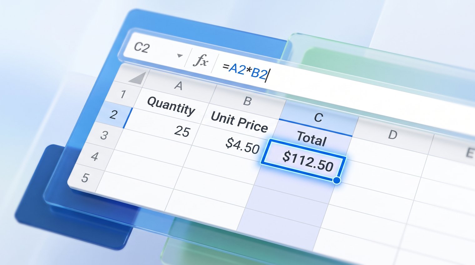
The core Excel multiplication formula is =A2*B2. Excel uses the asterisk symbol (*) for multiplication, not the letter x.
For example, if cell A2 contains a quantity of 4 and B2 contains a unit price of $12.50, enter =A2*B2 in C2. Excel returns 50, which is the line-item total.
Enter a Multiplication Formula Correctly
Click the cell where you want the answer to appear, type an equal sign, select or type the first cell reference, enter an asterisk, and then select or type the second cell reference. Press Enter to calculate it.
For instance, to multiply B2 by C2, type =B2*C2. You can click B2, type *, and click C2 instead of typing the references manually. This reduces typos when you are working in a large worksheet.
After pressing Enter, the active cell displays the result, while the formula bar displays the formula itself. If either source value changes later, Excel automatically updates the result.
Example: Calculate a Line-Item Total
Suppose an order sheet uses column B for quantity, column C for unit price, and column D for the total. If B2 contains 6 and C2 contains 14.25, enter this formula in D2:
=B2*C2
The result is 85.50. Format column D as Currency if you want Excel to display the dollar sign and two decimal places.
Copy the Formula Down a Column
You should not rewrite the same multiplication formula for every row. Once the formula is correct in the first row, copy it down the total column.
Select the formula cell, then point to the small square in its lower-right corner. This is the fill handle. Drag it down through the rows you need, or double-click it when an adjacent column contains a continuous list of data.
Excel adjusts relative references as it copies. A formula of =B2*C2 in row 2 becomes =B3*C3 in row 3, then =B4*C4 in row 4. You can also copy the first formula with Ctrl+C and paste it into the destination cells.
A common mistake is filling through blank rows or rows with inconsistent data. If a quantity is missing, text has been entered in a price column, or the list has a gap, inspect that row before assuming the formula failed.
Multiply a Range of Cells with PRODUCT
Use the PRODUCT function when you need to multiply more than two values together. Its basic syntax is:
=PRODUCT(A2:C2)
This multiplies every numeric value in A2, B2, and C2. For example, if those cells contain 2, 3, and 4, the result is 24.
You could write =A2*B2*C2 instead, and that is perfectly fine for a short, obvious calculation. PRODUCT is often easier to read when the formula contains a larger range or several groups of cells.
Use PRODUCT for Non-Adjacent Cells and Ranges
PRODUCT can also work with separate cells and ranges. For non-adjacent cells, use commas:
=PRODUCT(A2,C2,E2)
To multiply all values in two ranges, use:
=PRODUCT(A2:A5,C2:C5)
PRODUCT ignores text and empty cells, but it does not ignore zero. If any included numeric cell contains 0, the final result is 0. That is mathematically correct, but it can be surprising when a zero is being used as a placeholder for missing data.
Multiply an Entire Column of Values
There are two different tasks people mean when they say they want to multiply a column. The usual task is calculating a separate total for each row, such as quantity times price. For that, enter a formula like =B2*C2 and fill it down.
The less common task is finding one cumulative product from every number in a column. Use:
=PRODUCT(B2:B10)
This multiplies B2 through B10 into one result. It can be useful for compounding factors, probability calculations, or chained growth rates. It is generally not the right formula for sales sheets, invoices, or inventory lists, where each row should have its own total.
Multiply by a Fixed Number Without Breaking the Formula
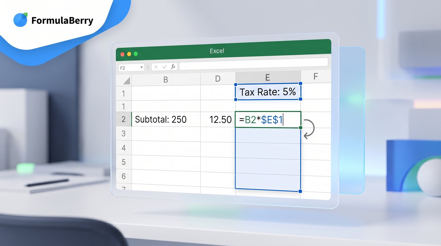
When every row must use the same multiplier, lock the multiplier cell with an absolute reference. For example, if quantities are in B2:B20 and a fixed rate is stored in E1, use:
=B2*$E$1
The dollar signs tell Excel to keep E1 fixed when you copy the formula down. In the next row, the formula becomes =B3*$E$1, not =B3*E2. For more advanced reference-building techniques, see this guide to the Excel ADDRESS formula.
You can use this for a fixed commission rate, tax rate, conversion factor, or discount multiplier. For example, if E1 contains 10%, =B2*$E$1 calculates 10% of the value in B2.
Tip: Press F4 while editing a cell reference to cycle through relative and absolute reference options. For a fixed multiplier, the usual choice is $E$1.
Multiply Prices, Quantities, and Percentages
A common pricing formula begins with quantity multiplied by unit price, then applies an adjustment such as a discount, tax, or markup. The important detail is how the percentage is stored. For more examples, see this guide to the Excel percentage formula.
If a cell contains 10%, Excel treats it as 0.10. If it contains the whole number 10, Excel treats it as ten, not ten percent. Formatting a value as Percentage is usually the clearest approach.
For a discount stored in D2, use:
=B2*C2*(1-D2)
If B2 is 5, C2 is $20, and D2 is 10%, the formula calculates $90. The original total is $100, and multiplying by 0.90 applies the 10% discount.
Add Tax or Markup to a Product Total
To add a fixed tax or markup rate stored in F1, use:
=B2*C2*(1+$F$1)
If F1 contains 8%, the formula multiplies the product total by 1.08. Multiplying by 1.08 adds 8%, while multiplying by 0.92 applies an 8% discount.
Do not multiply a total by 8% when your goal is to add tax. That returns only the tax amount. Use 1 + rate to calculate the tax-inclusive total.
Multiply Numbers Directly in an Excel Formula
For a one-off calculation, you can multiply numbers directly in a formula:
=12*5
You can also include an adjustment factor, such as =12*5*1.08 to add 8% to a total of 60.
Direct numbers are useful for quick checks, but cell references are better in a reusable worksheet. With references, anyone can change the inputs without editing the formula itself, and the values remain visible in the sheet.
Use Multiplication with IF When a Calculation Depends on a Condition
Use IF when a row should be multiplied only if it meets a condition. For example, if column A says whether an item qualifies, calculate the total only when A2 contains Yes:
=IF(A2="Yes",B2*C2,0)
If A2 is Yes, Excel multiplies B2 by C2. If it is anything else, the formula returns 0. Quotation marks are required around text conditions such as "Yes."
Returning 0 is often more useful than returning a blank because later Excel SUM formulas can include the result without special handling. Use an empty string, written as "", only when you truly need the cell to look blank.
Fix Common Excel Multiplication Formula Errors
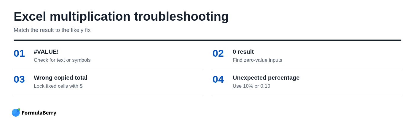
If a multiplication formula returns #VALUE!, Excel is usually trying to multiply text rather than numbers. Imported data is a frequent culprit: a price may look like $25.00 but be stored as text because it includes a currency symbol, a hidden space, or another nonnumeric character.
A result of 0 usually means at least one referenced cell is zero. It can also happen when a blank input is being treated as zero in the calculation. Check every cell referenced by the formula before changing the formula itself.
If the first formula works but copied rows are wrong, review your references. A cell that should remain fixed needs dollar signs, such as $E$1. A row-specific value should normally remain relative, such as B2 or C2.
Percentage errors are also common. If a formula produces a value ten times or one hundred times larger than expected, confirm whether the rate is stored as 10%, 0.10, or 10.
Check Whether a Number Is Stored as Text
Text-formatted numbers often align to the left by default, while regular numbers align to the right. You may also see a small green triangle in the cell corner or an error prompt indicating that a number is stored as text.
First, remove unnecessary spaces, currency characters, or imported labels from the source values. If you need to convert a clean text number, use =VALUE(A2) in a helper cell, then use the converted result in your multiplication formula. For a quick worksheet fix, Excel's "Convert to Number" option can also work when the error indicator appears.
Build Multiplication Formulas Faster from Plain-English Requests
When the calculation becomes more involved, state the logic before writing the formula. For example: "Multiply quantity by price, subtract the row's discount, then add 8% tax." That description makes it easier to identify which cells change by row and which rate must stay fixed.
You can use FormulaBerry to generate, explain, or correct Excel and Google Sheets formulas from a plain-English request. Describe the columns and calculation you need, then verify the proposed cell references against your worksheet.
Always test a new formula on one row with numbers you can calculate manually. Once the result is correct, fill it down the column.
Choose the Right Excel Multiplication Formula for the Job
Use * for ordinary cell-by-cell multiplication, such as =B2*C2. Use PRODUCT when one formula must multiply several cells or ranges. Use absolute references such as $E$1 whenever a tax rate, commission rate, or other fixed multiplier should not move as you copy the formula.
For most business worksheets, the dependable pattern is simple: keep inputs in separate cells, calculate each row with relative references, lock only the fixed rates, and verify the first result before filling down. If a more complex spreadsheet calculation is difficult to translate into a formula, FormulaBerry can help turn the requirement into a formula you can review and use.