A Google Sheets formula can be only a few characters long and still cause an hour of frustration. The problem is rarely the function itself. More often, the formula was built for the wrong range, the wrong match type, or an edge case nobody stated upfront.

A Google Sheets formula generator helps close that gap. Instead of remembering syntax from scratch, you describe the result you need, identify the relevant columns, and receive a formula you can inspect and paste into your sheet. Used well, it speeds up formula creation, explanation, and troubleshooting without replacing the need to check the result.

What a Google Sheets Formula Generator Does - and What It Cannot Do

An AI formula generator translates a plain-English spreadsheet request into a Google Sheets formula. It can also explain an existing formula in simpler language and suggest corrections when a formula returns an error or an unexpected result.

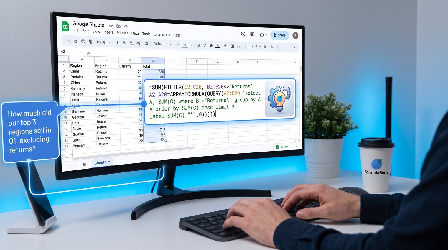
The basic workflow is straightforward: describe the outcome, provide the column or range context, state any conditions, and ask for a formula that fits the intended destination cell. For example: "In G2, calculate revenue in E2 minus discount in F2, but leave the cell blank if revenue is blank."

That is different from giving an AI access to a complete spreadsheet and expecting it to automatically clean bad data, design a reporting model, or determine whether your source records are factually correct. A formula generator can write a rule. It cannot know that a customer record was mislabeled, that a date was entered in the wrong year, or that your team's definition of "completed" changed last month.

Think of generated formulas as a strong first draft with a technical explanation available on demand. The formula may be syntactically valid while still applying the wrong business rule, so validation remains part of the job.

Quick start: describe the outcome, ranges, and edge cases

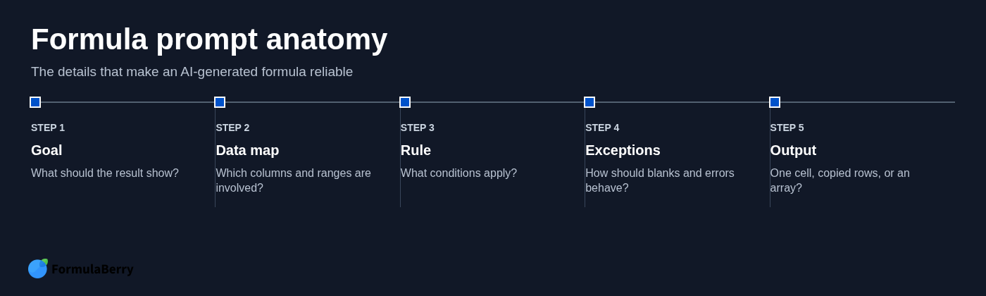
A useful request includes five pieces of information:

• Desired output: What should the formula return?
• Source data: Which columns, ranges, or sheets contain the inputs?
• Rule: What conditions determine the result?
• Exceptions: How should blanks, missing matches, and errors behave?
• Output shape: Do you need one result, a formula copied down rows, or a spilling array?

For example, ask: "In G2, calculate quantity in C2 multiplied by unit price in D2, minus the discount percentage in E2. Return blank when C2 or D2 is blank, and return the result for one row so I can copy it down."

A suitable formula is:

=IF(OR(C2="",D2=""),"",C2*D2*(1-E2))

Before filling it down, test it on a row with ordinary values, a blank quantity, and a zero discount. That quick check catches misunderstandings before they spread through hundreds of rows.

How to Write Prompts That Produce Usable Google Sheets Formulas

The quality of a generated formula depends heavily on the details in the request. "Calculate sales by month" is too vague: it does not say where sales live, what counts as a month, whether cancelled orders should be excluded, or whether the result should be a single number or a report table.

A reliable request follows a simple sequence: map the data, state the rule, define exceptions, and specify the output. You do not need to share sensitive customer records to do this. Column headers and a few anonymized sample rows are usually enough.

For example, replace names, emails, and account numbers with representative dummy values. The important part is preserving the data structure: whether dates are actual dates, whether revenue is numeric, and whether a status field contains values such as "Completed," "Pending," or "Cancelled."

Also mention spreadsheet conventions that can change formula syntax. Some locales use semicolons instead of commas as function argument separators. Date entries may be interpreted differently depending on regional settings. And a request that needs a fixed lookup range should say so, because absolute references such as $A$2:$D$100 behave differently from relative references that shift when copied down.

Specify the data layout before asking for a formula

State the sheet name, headers, exact ranges, whether the first row contains headers, and where the formula should go. If your data sits on a sheet named Orders, say that rather than assuming a generator can infer it.

Here is a much stronger request:

"On the Orders sheet, headers are in row 1. Column A contains order dates, B contains regions, E contains revenue, and F contains status. In Summary!B2, return total completed revenue for the region in A2 during the month selected in B1."

Output granularity matters just as much. Say whether you need:

• A single-cell result for a dashboard.
• A row-level formula beginning in a specific cell and copied down.
• A dynamic array that spills into empty cells automatically.

Without that instruction, a formula can be correct in isolation but unusable in the sheet where you intend to place it.

State the business rule and exceptions explicitly

Do not make a generator guess how to treat messy data. If duplicate IDs are possible, say whether you want the first match, the latest match, or every matching record. If a missing match should display "Not found" instead of an error, state that. If numeric-looking values may be stored as text, mention it.

Specific instructions lead to intentional function choices. For instance, asking to "show blank instead of an error if no matching record exists" points toward an error wrapper such as IFERROR. Asking for "all completed orders in the selected region" points toward FILTER, not a single-result lookup. Asking for "return blank when either input is missing" calls for an IF condition before the main calculation.

A practical request might read: "Find the first exact product ID match. If no match exists, return 'Missing product.' Do not use approximate matching. Product IDs in both columns are text." That is far safer than simply asking for a lookup formula.

Generate Everyday Calculations First

Start with small, transparent calculations. They are easy to verify manually and help you build confidence in how formulas reference cells, handle blanks, and behave when copied through a table.

For each generated formula, check one normal row with a calculator or manual arithmetic. Then test a blank input and an unusual value, such as zero. Those three cases reveal most early mistakes.

Add, subtract, multiply, and divide values safely

Suppose a sales table uses column B for quantity, C for unit price, D for discount rate, and E for cost per unit. You want net revenue in F2 and gross margin in G2.

Plain-English request: "In F2, multiply quantity in B2 by unit price in C2, reduce the result by discount rate in D2, and return blank when quantity or price is blank."

=IF(OR(B2="",C2=""),"",B2*C2*(1-D2))

The formula calculates gross sales, then multiplies by the remaining percentage after the discount. If D2 contains 10%, the multiplier is 90%, or 0.9.

For margin, ask: "In G2, calculate net revenue in F2 minus quantity in B2 multiplied by cost per unit in E2. Leave blank if F2 is blank."

=IF(F2="","",F2-(B2*E2))

Division needs extra protection. A Google Sheets divide formula such as =C2/B2 produces #DIV/0! when B2 is zero or blank. If you want a blank rather than an error, use:

=IF(OR(B2="",B2=0),"",C2/B2)

Validate this with a normal denominator, a zero denominator, and a blank denominator. Do not use IFERROR as a blanket fix when you can identify the actual condition; explicit logic is easier to maintain.

Calculate percentages, totals, and averages

A percentage is a calculation first and a display format second. If actual revenue is in B2 and target revenue is in C2, the attainment percentage is:

=IFERROR(B2/C2,"")

Format the result cell as a percentage in Google Sheets. A displayed value of 75% is stored as 0.75, which matters when you use it in later calculations.

For a total, use:

=SUM(E2:E100)

For an average, use:

=AVERAGE(E2:E100)

One common reporting mistake is adding percentages when the real question is percentage of a total. If B2 contains a region's revenue and B2:B5 contains all region revenues, use:

=IFERROR(B2/SUM($B$2:$B$5),"")

The fixed dollar signs keep the total range anchored when you copy the formula down. Adding 20%, 30%, and 40% produces 90%, but that total only has meaning if those percentages share the same denominator and are meant to be additive.

Generate Conditional Counting and Summing Formulas

Once a spreadsheet needs answers such as "How many completed orders did we receive?" or "What was revenue for the West region this month?" simple arithmetic is no longer enough. Conditional aggregation functions count, sum, or average only the records that meet stated criteria.

Use COUNTIF and SUMIF for one condition. Use COUNTIFS, SUMIFS, and AVERAGEIFS when the answer depends on two or more conditions.

Count records that match a condition

Suppose order status is in F2:F500. To count completed orders, use this COUNTIF formula in Google Sheets:

=COUNTIF(F2:F500,"Completed")

To count leads from a specific source in column C, where the source name is entered in H2, use:

=COUNTIF(C2:C500,H2)

Wildcards can help with partial text matching. For example, =COUNTIF(C2:C500,"*Referral*") counts cells containing the word Referral. Use wildcards carefully: a partial match can include labels you did not intend to group together.

Dates need particular care. If dates are true date values in A2:A500, count records in January 2026 with:

=COUNTIFS(A2:A500,">="&DATE(2026,1,1),A2:A500,"

Avoid matching dates by their displayed text whenever possible. Also inspect inconsistent labels and hidden spaces. "Completed", "completed", and "Completed " may not behave as one category in every formula approach.

Generate Lookup Formulas Without Common Matching Mistakes

Lookups are valuable because they connect tables: an order sheet can retrieve a product category, price, account manager, or customer segment from a separate reference table. They are also easy to get wrong when the request does not specify match behavior.

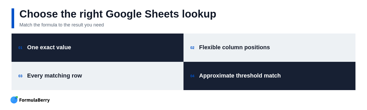
Before generating a lookup, decide whether you need one exact value, an approximate value based on thresholds, or every record that matches. Those are different jobs and should not be solved with the same formula by default.

Use VLOOKUP for simple left-to-right tables

VLOOKUP searches the first column of a selected table range and returns a value from a column to its right. For a simple product table where product ID is in Products!A2:A100 and category is in Products!C2:C100, retrieve the category for the product ID in A2 with:

=IFERROR(VLOOKUP(A2,Products!$A$2:$C$100,3,FALSE),"Missing product")

The final FALSE requests an exact match. That is the right default for IDs, email addresses, SKUs, and other keys that must match precisely. Omitting it can allow approximate behavior, which is dangerous unless your table is deliberately sorted for threshold matching. For more examples and troubleshooting, see this guide to the VLOOKUP formula in Google Sheets.

VLOOKUP has a structural limitation: the lookup key must be in the first column of the selected range, and it can only return values to the right. If your table layout does not meet those requirements, choose a more flexible method rather than rearranging a live dataset just to satisfy a formula.

Use XLOOKUP or INDEX/MATCH when the table structure demands it

XLOOKUP is often clearer because you specify the lookup range and return range separately. For the same product example:

=XLOOKUP(A2,Products!$A$2:$A$100,Products!$C$2:$C$100,"Missing product",0)

The final match mode of 0 requests an exact match. Unlike VLOOKUP, XLOOKUP can return a value from a column to the left or right of the key column.

INDEX/MATCH remains useful in established spreadsheets and in situations where that pattern is already part of your team's formulas. An equivalent formula is:

=IFERROR(INDEX(Products!$C$2:$C$100,MATCH(A2,Products!$A$2:$A$100,0)),"Missing product")

The decision rule is simple: use VLOOKUP for stable, left-to-right reference tables; use XLOOKUP when separate lookup and return ranges make the formula clearer; use INDEX/MATCH when you need to work within an existing pattern or want explicit control over the match position.

Return every matching row with FILTER instead of forcing a lookup

A lookup normally returns one value. If your real requirement is "show every completed order for the selected customer," use FILTER instead.

For example, to return all rows in A2:F500 where the customer in column C matches H2 and the status in F is Completed:

=IFERROR(FILTER(A2:F500,C2:C500=H2,F2:F500="Completed"),"No matching orders")

This formula spills matching rows into the cells below and beside the formula cell. Make sure that output area is empty.

When writing your request, distinguish "return the first matching product category" from "return all matching order rows." The first suggests a lookup; the second requires a dynamic result set.

Create Array Formulas for Entire Columns and Dynamic Results

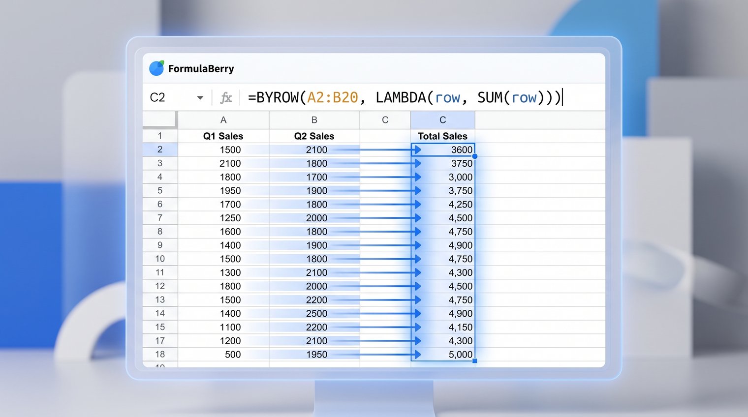
Copied-down formulas and array formulas solve related but different problems. A copied formula calculates one row at a time and must be filled into each row. An array formula can calculate many rows from a single starting cell and spill results automatically.

This changes the request you give a Google Sheets formula generator. You need to specify the output area, whether the formula should include a header, and what should happen for future rows added to the dataset.

When to use ARRAYFORMULA

Use ARRAYFORMULA when the same row-level calculation should apply across a full column. Suppose column B contains quantity, C contains unit price, and you want revenue in D with a header included:

=ARRAYFORMULA({"Revenue";IF((B2:B="")+(C2:C=""),"",B2:B*C2:C)})

The braces create a two-part vertical output: the header "Revenue" followed by the calculated values. The IF condition prevents empty source rows from generating unwanted zeros.

Place this formula at the top of an empty destination column. It needs room to spill downward, and existing values in that column will block the result. Open-ended ranges such as B2:B are convenient for growing datasets, but they can also make a sheet slower when used carelessly across many complex formulas.

Ask for an array formula explicitly: "Put a single formula in D1 that adds a Revenue header and calculates quantity times unit price for every populated row, leaving blank rows empty." For more examples, see this guide to the ARRAYFORMULA in Google Sheets.

Use dynamic-array functions for cleaner transformations

Google Sheets also has functions designed to generate dynamic lists and tables. FILTER returns only rows meeting conditions, UNIQUE removes repeated values, SORT orders a result, and QUERY can filter, group, and summarize tabular data.

The right function depends on the output shape. A unique list of regions is different from a filtered order list, and both are different from a grouped monthly sales summary.

For a sorted unique region list from B2:B500:

=SORT(UNIQUE(FILTER(B2:B500,B2:B500"")))

For a dynamic report, do not just ask for "a formula using QUERY." Explain the desired table: its columns, grouping level, filters, sorting order, and treatment of empty results. Function names are implementation details; the report shape is the actual requirement.

Ask an AI to Explain an Existing Google Sheets Formula

Formula generation is only half the value. Many spreadsheet users inherit workbooks containing formulas that are technically correct but impossible to understand at a glance. A formula assistant can translate that logic into plain English before you edit it.

Ask for both a concise summary and a function-by-function breakdown. The summary tells you the formula's business purpose; the breakdown lets you inspect how it reaches that result.

For example, instead of pasting a formula and asking "What does this do?", ask: "Explain this formula in beginner-friendly language. Identify each referenced range, explain every condition, and tell me what result appears when no match is found. Do not rewrite it yet."

That last instruction matters. A simpler-looking formula is not automatically equivalent. First confirm what the original formula is intended to return, then ask whether a simpler version would preserve that behavior.

Request explanations at the right level of detail

Choose the explanation depth based on the task. For quick review, ask for a one-paragraph summary. For auditing, request an annotated breakdown of each nested function. For a very long formula, ask about only the portion you need to change.

Include context about named ranges and cell references. A reference such as $B$2 is locked in both row and column when copied. B$2 locks only the row, while $B2 locks only the column. These small differences often explain why a formula works in one row and fails after being filled elsewhere.

Also ask what error wrappers are hiding. An IFERROR can make a report look clean while concealing missing data or a broken lookup. That may be appropriate, but it should be an informed choice rather than an accident.

Fix Broken or Incorrect Formulas Systematically

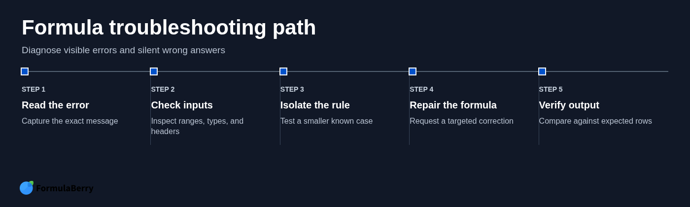
A Google Sheets formula checker is most useful when it helps separate two problems: formulas that visibly fail and formulas that return a plausible but wrong answer. The first category usually produces an error code. The second is more dangerous because nothing looks broken.

When requesting a correction, provide the formula, the exact error message or wrong result, the relevant headers and ranges, and the output you expected. That gives the assistant enough context to suggest a targeted repair rather than merely swapping functions.

Diagnose errors such as #N/A, #VALUE!, #REF!, and #DIV/0!

#N/A usually means a lookup or match did not find the requested value. Check whether the key exists in both tables, whether one key is text while the other is numeric, and whether invisible spaces are present. The repair may be an exact-match correction, data cleanup, or a deliberate fallback message.

#VALUE! often points to incompatible input types or an invalid operation. A calculation may be attempting to multiply text, or a function may receive an argument in the wrong format. Inspect the actual cell values rather than relying only on how they look on screen.

#REF! means the formula points to an invalid reference or cannot expand into occupied cells. This often follows deleted columns, moved ranges, or a blocked array spill area.

#DIV/0! means the denominator is zero or blank. Decide whether a zero denominator is expected and should return blank, zero, or a label such as "No target." The correct response depends on the report's meaning.

A well-formed correction request is: "This formula in G2 returns #N/A: [formula]. It looks up the product ID from A2 against Products!A2:A100 and should return the category from Products!C2:C100. A2 contains 1034, and the expected category is Office. Explain the cause and provide a corrected formula."

Catch silent logic errors that show no error message

Not every bad formula produces an error. A total can be wrong because numbers are stored as text, a criteria range is one row out of alignment, a relative reference shifted during copying, or a lookup silently uses approximate matching.

As covered in the lookup section, approximate matching is especially risky for IDs and codes. Use exact-match instructions unless you are intentionally matching a sorted threshold table, such as a commission-rate schedule.

Create a small known-answer test set before applying a generated formula across a live sheet. Include records that should qualify, records that should not, blank values, duplicate keys, and at least one boundary case. Write down the expected answer first, then compare the formula output.

This is not overkill. A formula that is wrong in a quiet, consistent way can make a dashboard look credible while distorting every decision based on it.

Worked Example: Build a Reliable Sales Summary From Raw Data

Consider a compact Orders sheet with these columns: A: Order Date, B: Region, C: Rep, D: Product, E: Revenue, and F: Status. You want a summary for a selected month and region without manually filtering the raw table every time.

The goal is to return completed revenue for the selected region, plus that region's share of total completed revenue for the selected month. This example focuses on the formula design and validation process; it is not a claim that the formulas have been run against a particular live spreadsheet.

Define the requested report and expected output

Set up a Summary sheet where B1 contains any date in the selected month and B2 contains the selected region. The report should show:

• Completed revenue for the selected region and month.
• Total completed revenue across all regions for that month.
• The selected region's percentage of that monthly total.

State the assumptions before generating formulas: blank order dates should be ignored, cancelled orders should not count, the status must equal "Completed," and an empty result should display 0 for revenue figures. The percentage should be blank when there is no monthly completed revenue, because a share of zero total is not meaningful.

A precise request could be: "On Summary, B1 contains a date within the reporting month and B2 contains the region. In B4, sum revenue from Orders!E2:E where the order date in Orders!A2:A is within B1's month, region in Orders!B2:B matches B2, and status in Orders!F2:F is Completed. Ignore blank dates and return 0 when there are no qualifying rows."

Generate, inspect, and validate the formulas

For selected-region completed revenue, one formula is:

=SUMIFS(Orders!E2:E,Orders!A2:A,">="&EOMONTH($B$1,-1)+1,Orders!A2:A,"

The first date criterion starts on the first day of B1's month. The second stops before the first day of the next month. This approach handles dates with times more reliably than trying to match a formatted month label.

For total completed revenue in the same month, remove the region criterion:

=SUMIFS(Orders!E2:E,Orders!A2:A,">="&EOMONTH($B$1,-1)+1,Orders!A2:A,"

If selected-region revenue is in B4 and monthly total is in B5, the share formula in B6 is:

=IF(B5=0,"",B4/B5)

Format B6 as a percentage. Now validate in stages rather than trusting the final number immediately. First filter the Orders sheet manually to the chosen date range and status. Add the revenue values for the selected region with a calculator or temporary SUM. Then compare that result to B4. Next, remove the region filter and compare the all-region total to B5.

A syntactically valid formula can still be logically wrong. For example, if the status criterion is omitted, cancelled revenue enters the report. If the date conditions use the wrong month cell, the summary may be consistently off by one period. Testing intermediate totals makes those errors visible.

Choose a Google Sheets Formula Generator Based on Your Task

Formula generators are not interchangeable just because they can produce formulas. Compare them by the task you actually need completed: formula generation, plain-English explanation, correction help, automation needs, and learning support.

1. FormulaBerry

FormulaBerry is a practical fit for users who want natural-language assistance with Google Sheets or Microsoft Excel formulas. You can describe the spreadsheet outcome, receive a custom formula, and then ask for an explanation or correction when the result needs clarification.

That create-explain-fix workflow is useful for reports, budgets, and routine analysis where the blocker is formula logic rather than a need for a full spreadsheet application. It is particularly helpful when you need to understand a formula before putting it into a shared workbook.

2. SheetFormula

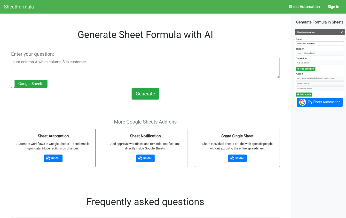
SheetFormula is positioned as an AI formula generator with an automation-oriented angle. When comparing it with a formula-focused assistant, assess whether your immediate need is simply creating and understanding a formula or whether your workflow also calls for row- or sheet-level automation.

Those are related needs, but they are not identical. A buyer who only needs to build, explain, and repair formulas should evaluate the clarity of the formula request and output experience first.

3. Better Sheets

Better Sheets may suit readers who value formula education and guides alongside a generator. Learning resources can help you recognize common patterns and improve long-term spreadsheet confidence.

Still, educational content and on-demand formula generation solve different problems. If you have an urgent reporting task, prioritize how easily you can provide context, review the generated formula, and get help interpreting or correcting it.

Protect Data and Verify AI-Generated Formulas Before Using Them

A free Google Sheets formula generator online can be useful, but convenience should not lead to careless data sharing. Remove personal information, account numbers, confidential pricing, and other sensitive values from requests whenever possible. Share headers, ranges, and anonymized sample rows instead.

Before entering business data into any tool, review its data-handling terms and make sure the level of access fits your organization's requirements. A formula request rarely needs an entire export of customer data.

Then validate the generated result with a short checklist:

• Compare key outputs to a manual calculation or known answer.
• Test blank cells, zero values, missing matches, and duplicate records.
• Confirm that criteria and sum ranges begin and end on the same rows.
• Check which references should remain fixed when copied.
• Verify that array formulas have an empty spill area.
• Save a prior version or copy the original formula before replacing it.

AI output is a draft to inspect, not proof that the business logic is correct. The more important a number is to a budget, forecast, or client report, the more deliberately it should be tested.

Get Better Google Sheets Formulas With Clear Requests and Fast Validation

Google Sheets formulas become much easier when you stop starting with function names and start with the result you need. Describe the data layout, rule, exceptions, and output shape, then inspect the generated formula against known records.

The most useful habit is a simple loop: create the formula, explain the logic, test the result, and correct it when the evidence says it is wrong. That process works for a basic percentage just as well as a dynamic sales report.

If you want help turning a plain-English spreadsheet task into a formula you can review and refine, try FormulaBerry for Google Sheets and Excel formula generation, explanation, and correction.