Long URLs make an otherwise useful Google Sheet hard to scan. Worse, a URL stored as plain text may look like a link without giving your team a reliable, labeled click target.

The Google Sheets HYPERLINK formula fixes that. You can use it to create clean web links, build links from IDs in your data, jump between worksheets, or launch an email from a contact list.

Use the HYPERLINK formula to create a clickable link

The basic Google Sheets hyperlink formula is:

=HYPERLINK(url, [link_label])

The first argument, url, is the destination. The optional second argument, link_label, is the text people see and click in the cell.

For example:

=HYPERLINK("https://example.com","Visit Example")

After you press Enter, the cell displays Visit Example as a clickable link. The destination must be a valid URL or another supported destination, such as an internal location in the same spreadsheet, for the link to work correctly.

Build your first hyperlink from fixed text

Click an empty cell, paste this formula, and press Enter:

=HYPERLINK("https://example.com","Open example site")

The cell should now display Open example site. Click it to open the destination. This is the simplest Google Sheets hyperlink formula example because both the URL and visible text are fixed inside the formula.

The label is optional. If you leave it out, Google Sheets uses the destination itself as the clickable value. That can be useful, but it is rarely the best choice for a report or tracker.

Use a URL as the visible link text

Use this version when you want readers to see the complete destination:

=HYPERLINK("https://example.com")

Showing the full URL makes sense in a link inventory, audit sheet, or a record where the exact destination matters. It is less useful in client-facing reports, where long URLs quickly make columns difficult to read.

Use a custom label for a cleaner sheet

For most working sheets, use a short label instead:

=HYPERLINK("https://example.com","Open product page")

Labels such as View invoice, Open brief, or See source let readers understand the action without parsing a long URL. This is especially helpful in project trackers, content calendars, budgets, and status reports.

Turn URLs already in your sheet into clickable links

Often, the URL already exists in your spreadsheet. For example, column A may contain source pages, customer portals, product pages, or document links imported from another system.

If the first URL is in cell A2, enter this in B2:

=HYPERLINK(A2,"Open link")

Press Enter, then drag the fill handle down the column to apply the formula to the remaining rows. Each row in column B will use the URL from the matching row in column A.

A URL stored as plain text in A2 is just data. The HYPERLINK formula in B2 turns that data into a deliberate clickable link with a readable label. Do not assume every URL-looking value has already been converted into a working hyperlink.

Create dynamic hyperlink labels and destinations from cells

The real value of HYPERLINK appears when the destination changes row by row. You can combine fixed text with cell values using the ampersand (&) operator.

Suppose column A contains item IDs and column B contains product names. This formula creates a unique product URL and a label that changes with the name:

=HYPERLINK("https://example.com/item/"&A2,"View "&B2)

If A2 contains SKU-1042 and B2 contains Blue Notebook, the formula points to https://example.com/item/SKU-1042 and displays View Blue Notebook.

Before filling a dynamic formula down hundreds of rows, test it on one or two records. A common mistake is referencing the wrong source column, which can produce valid-looking links that lead to the wrong page.

Link to a page or record ID stored in a cell

When your sheet holds IDs from a CRM, ecommerce system, or dashboard, construct the link around the ID. If A2 contains a customer record ID, use a pattern like this:

=HYPERLINK("https://portal.example.com/customers/"&A2,"Open customer record")

The fixed part of the URL stays the same. Only the value from A2 changes for each row. This is far more maintainable than pasting hundreds of individual links by hand.

Use a dynamic label that updates with your data

You can also build the label from the cells that describe each record:

=HYPERLINK(A2,"Open "&B2)

Here, A2 contains the destination URL and B2 contains a name, title, or ID. If the name changes later, the clickable label updates automatically, which keeps a live tracker understandable.

If you need help translating a description such as "make a link from the ID in column A and name it with column B" into the exact formula, Google Sheets Formula Generator: Create, Explain, and Fix Formulas can help you generate, explain, or correct it.

Link to another sheet, cell, or range in the same spreadsheet

External websites are not the only possible destinations. You can create a Google Sheets hyperlink to another sheet, cell, or range within the same spreadsheet.

Use a destination beginning with #gid=, followed by the destination worksheet's ID. To jump directly to a cell, add &range=:

=HYPERLINK("#gid=123456789&range=B2","Go to details")

Replace 123456789 with the actual gid for the worksheet you want to open. To find it, open the destination tab and look at the spreadsheet URL in your browser. The relevant fragment appears after gid=. If you want to direct people to a particular location, add a range such as A1, B2, or A1:D20.

The gid identifies the worksheet, not its visible name. That matters when sheet names contain spaces, punctuation, or get renamed. Use the gid from the destination tab rather than trying to build an internal link from the tab name alone.

Make a table of contents that jumps to each worksheet

A workbook with many tabs benefits from a simple navigation page. On a Dashboard sheet, create labels such as Open Data, View Monthly Summary, and Go to Archive, each pointing to the appropriate worksheet gid.

This is a practical table of contents for recurring reports, operating budgets, and team trackers. It saves people from hunting through a crowded row of worksheet tabs every time they need a source table.

Create email, phone, and prefilled-action links

HYPERLINK also works with action-based destinations. For a contact list, a mailto: link is often the most useful option.

If A2 contains an email address, use:

=HYPERLINK("mailto:"&A2,"Email contact")

Clicking the label opens the user's default email application or webmail handler with the address populated. This works well in outreach lists, supplier directories, and customer follow-up sheets.

You can create a phone link with a tel: destination:

=HYPERLINK("tel:"&A2,"Call contact")

Phone links are most useful on smartphones, where the device can hand the number to its calling app. On desktop, the result depends on the installed apps and browser settings, so do not use a phone link as the only way to display a number.

Make sure your hyperlink is actually clickable

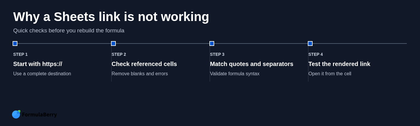
When a Sheets link is not working, start with the destination rather than rebuilding everything. A complete external URL should normally begin with a supported scheme such as https://.

For example, this is a complete destination:

=HYPERLINK("https://example.com","Open site")

By contrast, example.com may not behave consistently when used as a formula destination. Include the full scheme, especially when you are building URLs with cell references.

Also check for invisible problems in source data. Extra spaces, an empty ID, or an error in a referenced cell can create a broken result. If you are joining text with &, inspect the final URL in a separate cell first:

="https://example.com/item/"&A2

Once that output looks correct, place the same expression inside HYPERLINK.

Other common issues include:

• Missing quotation marks: Fixed text and URLs must be enclosed in quotes. Cell references should not be quoted.
• Wrong argument separator: Some Google Sheets locales use semicolons instead of commas. If a formula errors immediately, replace commas with semicolons.
• Invalid references: Confirm that the URL cell contains a value and that your formula points to the intended row.
• Plain-text URLs: A value that looks like a link is not necessarily a formula-created clickable link with the behavior and label you expect.

Add hyperlinks without a formula when that is the better option

You do not need HYPERLINK for every link. For a one-off link in a single cell, select the cell and use the Insert link command. On desktop, you can also use the keyboard shortcut for inserting a link, then enter the destination and display text.

Manual insertion is the better option when you are editing a single note, document reference, or exception row. HYPERLINK is better when links need to repeat, update from source data, or follow a consistent pattern across many rows.

On mobile, select the cell and use the Google Sheets app's insert-link option for a simple manual link. You can enter formulas on mobile too, but building and checking longer concatenated formulas is generally easier on a desktop screen.

Use HYPERLINK formulas confidently in larger sheets

Keep raw URLs, record IDs, and other source values in dedicated columns. Then place the HYPERLINK formula in a separate output column with a clear header such as Open record, Source link, or View page.

Use meaningful labels instead of generic text wherever possible. A column full of links labeled only Click here becomes confusing as soon as someone filters, exports, or shares the sheet. Labels like View Q3 invoice or Open Acme profile preserve context.

Test a single row before autofilling. Confirm both the rendered label and the destination, then copy the formula down. If you are building row-based references in a larger sheet, the Google Sheets ROW Formula: Number Rows and Build References guide may also help.

For formulas with several cell references, nested logic, or unusual destination patterns, describe the sheet structure and desired result to FormulaBerry. It can help you generate the formula, explain what an existing formula does, or identify why a link formula is failing.

Choose the right link method for your Google Sheet

Use HYPERLINK when the link should be reusable, generated from data, or displayed with a consistent label. Use internal #gid links when you need fast navigation between worksheets. Use Insert link when you are making a one-off manual edit.

The most useful default formula is often simple: keep the URL in one column and use =HYPERLINK(A2,"Open link") in the next. When your links need to be custom or dynamic, describe your columns and desired label to FormulaBerry for help building the exact formula.