
A Google Sheets IFNA VLOOKUP formula replaces a missing-match #N/A error with a message, blank, or other intentional value. The standard pattern is =IFNA(VLOOKUP(search_key, range, index, FALSE), value_if_na), and it is the cleanest way to handle expected lookup misses without hiding unrelated formula errors.
That distinction matters. A missing product ID may be normal and worth flagging as "Not found," while a broken range reference is a problem you should see and fix.
The IFNA VLOOKUP formula in Google Sheets
Use IFNA around VLOOKUP when you want to replace only the #N/A result that occurs when Google Sheets cannot find a match. The core formula is:
=IFNA(VLOOKUP(search_key, range, index, FALSE), value_if_na)
In this formula, VLOOKUP searches for a value in the first column of a selected range and returns a value from another column in the same row. IFNA steps in only when that search returns #N/A. For more on the lookup function itself, see VLOOKUP Formula in Google Sheets: How to Use and Fix It.
The final argument, FALSE, requests an exact match. For product IDs, customer IDs, SKUs, employee codes, names, and most lookup tables, exact matching is usually the right choice. Approximate matching can return the wrong row when the source data is not sorted precisely, so it is not a safe default for everyday reports.
How IFNA and VLOOKUP work together
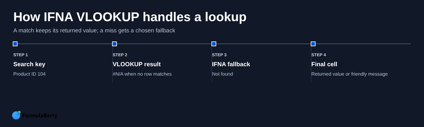
Google Sheets evaluates the VLOOKUP first. If it finds a matching row, IFNA returns the value VLOOKUP found. If VLOOKUP cannot find the search key and returns #N/A, IFNA returns your chosen fallback instead.
For example, a product catalog might contain Product ID 103 but not Product ID 104. A lookup for 103 can return its price, while a lookup for 104 can display "Not found" rather than an error.
A blank result and a missing match are not the same thing. If VLOOKUP finds a row but the return cell in that row is empty, the formula returns a legitimate blank. IFNA does not replace it because the lookup itself succeeded. That behavior is useful when an empty return value has a different meaning from "this record does not exist."
IFNA is also more precise than broad error handling. It deals with the expected absence of a matching record while leaving errors such as #REF!, #VALUE!, and formula parse errors visible for investigation.
Build an IFNA VLOOKUP formula step by step
Suppose the product ID you want to find is in cell A2. Your catalog is in columns H through J, where column H contains product IDs, column I contains product names, and column J contains prices.
To return the price, use:
=IFNA(VLOOKUP(A2,$H$2:$J$100,3,FALSE),"Not found")
- A2 is the search key: the product ID entered or listed in your results table.
- $H$2:$J$100 is the catalog range. Product IDs must be in column H because VLOOKUP searches the first column of its range.
- 3 tells VLOOKUP to return the value from the third column in that range, which is column J.
- FALSE requires an exact product ID match.
- "Not found" is the value IFNA returns when the product ID is absent from the catalog.
The dollar signs make the catalog reference absolute. When you fill the formula down from row 2 to row 3, A2 correctly changes to A3, but the catalog remains $H$2:$J$100. Without absolute references, the lookup range shifts down as well, which can cause valid records to disappear from the searchable range.
Choose a fallback value that works in downstream calculations
Your fallback should match how the result will be used. Use text such as "Not found" in a review-oriented report where someone needs to investigate missing IDs. Use an empty string, written as "", when you want a cleaner customer-facing display or a report that should stay visually uncluttered.
Do not automatically use 0. A zero price, zero quantity, or zero balance can be a real business value, so replacing missing records with 0 may quietly distort totals and decisions. If zero is genuinely the correct interpretation of no match, use it; otherwise, preserve the distinction.
Copy-ready IFNA VLOOKUP examples
These examples all use the same catalog structure: product IDs in H2:H100 and prices in J2:J100. Adapt the range and return-column number to match your own sheet.
Return a message when an ID is missing
=IFNA(VLOOKUP(A2,$H$2:$J$100,3,FALSE),"Product not found")
This formula returns the matching price when the ID in A2 exists. If it does not, the cell displays "Product not found," making the exception clear to anyone reviewing the sheet.
Return a blank cell instead of #N/A
=IFNA(VLOOKUP(A2,$H$2:$J$100,3,FALSE),"")
Use this version when missing results should not clutter a dashboard, invoice template, or formatted output. Remember that the cell is not truly empty from a formula perspective; it contains a formula that returns an empty string.
Use a numeric fallback carefully
=IFNA(VLOOKUP(A2,$H$2:$J$100,3,FALSE),0)
This is appropriate only when a missing match really should be treated as zero, such as an optional charge that has no applicable rate. If the difference between a true zero and an absent catalog record matters, add a separate status column:
=IFNA(VLOOKUP(A2,$H$2:$J$100,3,FALSE),"Missing")
That gives you a visible audit trail while allowing the price or quantity column to remain suitable for calculations.
Why your IFNA VLOOKUP still returns an error
IFNA does not fix every VLOOKUP issue. It only catches #N/A, so an error that remains visible is often telling you exactly what needs repair.
A #REF! error can mean the column index asks for a column outside the selected range. For instance, requesting column 3 from a two-column lookup range will fail. A #VALUE! or formula parse error often points to incorrect syntax, misplaced quotes, or an invalid argument.
Also check that the selected range includes both the lookup column and the return column. If you need to search product IDs in H and return prices from J, the range must begin in H and extend through J. Selecting only H:I makes it impossible to return a value from J.
Finally, confirm that you are using FALSE for an exact match. Approximate VLOOKUP can produce misleading results, particularly with unsorted IDs or text-based codes.
Check for hidden spaces and mismatched data types
Two values can look identical and still fail an exact match. A leading space in one product code, a trailing space copied from another system, or a number stored as text can prevent VLOOKUP from finding the row.
For text values with stray whitespace, TRIM can help:
=IFNA(VLOOKUP(TRIM(A2),$H$2:$J$100,3,FALSE),"Product not found")
Be deliberate when normalizing number-versus-text IDs. Converting values can be useful for purely numeric identifiers, but it is not a universal repair. An ID such as 00124 may need to remain text because its leading zeros are meaningful.
Make sure the lookup column is first in the range
VLOOKUP works left to right. The value you search for must appear in the first column of the range you provide, and VLOOKUP can only return columns to its right.
If your needed return value sits to the left of the lookup column, rearranging the data may be impractical. In that case, consider MATCH Formula in Google Sheets: Find Positions and Return Values with INDEX, or Google Sheets XLOOKUP, which do not have VLOOKUP's left-to-right limitation.
Use IFNA VLOOKUP with multiple criteria
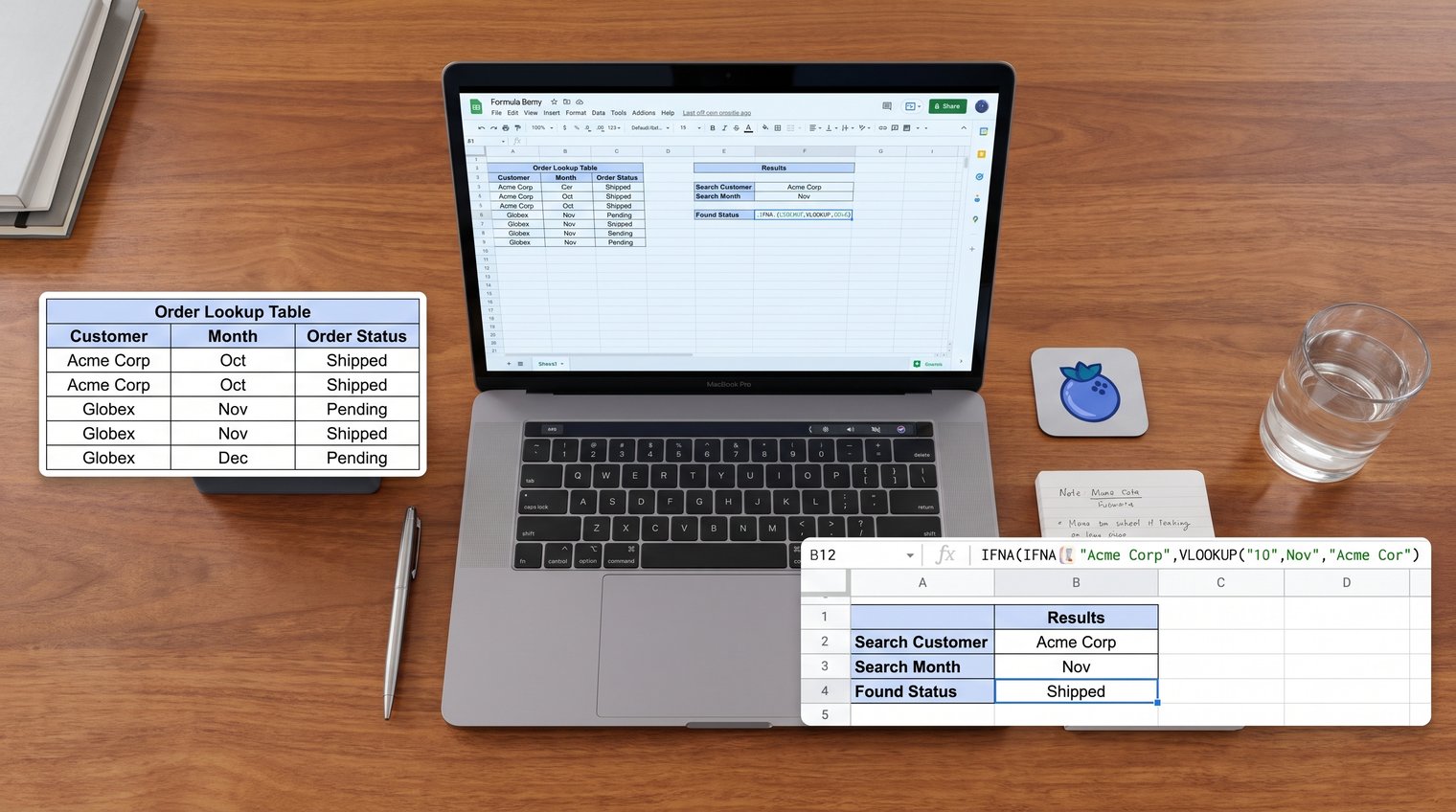
VLOOKUP accepts one search key, so a multiple-criteria lookup needs a combined key. This is useful when an order should match both a customer and a month, or when a price depends on both a product code and a region.
Assume A2 contains the customer, B2 contains the month, and the Orders sheet has customer names in column A, months in column B, and order status in column C. You can combine customer and month on both sides of the lookup:
=IFNA(VLOOKUP(A2&"|"&B2,{Orders!A2:A&"|"&Orders!B2:B,Orders!C2:C},2,FALSE),"No matching order")
The vertical bar acts as a separator, creating keys such as Acme Co|January. Choose a delimiter that is unlikely to appear in your actual data. If source values might contain a vertical bar, choose another character or use a helper-column approach. For more background on formulas that process ranges and return multiple results, see Array Formula in Google Sheets: Examples and How to Use It.
In a shared workbook, a helper column is often easier to audit. Add a combined key column to the Orders sheet, then use a standard IFNA VLOOKUP against that visible column. The formula may be less compact, but future editors can understand and troubleshoot it faster.
When to use IFNA instead of IFERROR
Use IFNA when a missing record is the expected condition you want to handle. Use IFERROR only when you have considered every possible error and the same fallback is appropriate for all of them.
| Purpose | Formula |
|---|---|
| Handle only a missing lookup match | =IFNA(VLOOKUP(A2,$H$2:$J$100,3,FALSE),"Not found") |
| Hide any error from the formula | =IFERROR(VLOOKUP(A2,$H$2:$J$100,3,FALSE),"Not found") |
The second formula may look convenient, but it can conceal a broken column index, invalid range, or other data issue behind the same friendly message. For exact-match VLOOKUPs, IFNA is usually the better default because it handles the normal "not found" outcome without masking problems that need attention.
Keep missing matches useful, not invisible
A reliable Google Sheets IFNA VLOOKUP formula combines three choices: an exact-match VLOOKUP, a fallback that fits the report, and a quick check for errors other than #N/A. That approach keeps expected missing IDs readable while preserving the warning signs of a genuinely broken formula.
If you need help building, explaining, or correcting a Google Sheets formula from a plain-English request, FormulaBerry can help generate a formula you can adapt to your spreadsheet.