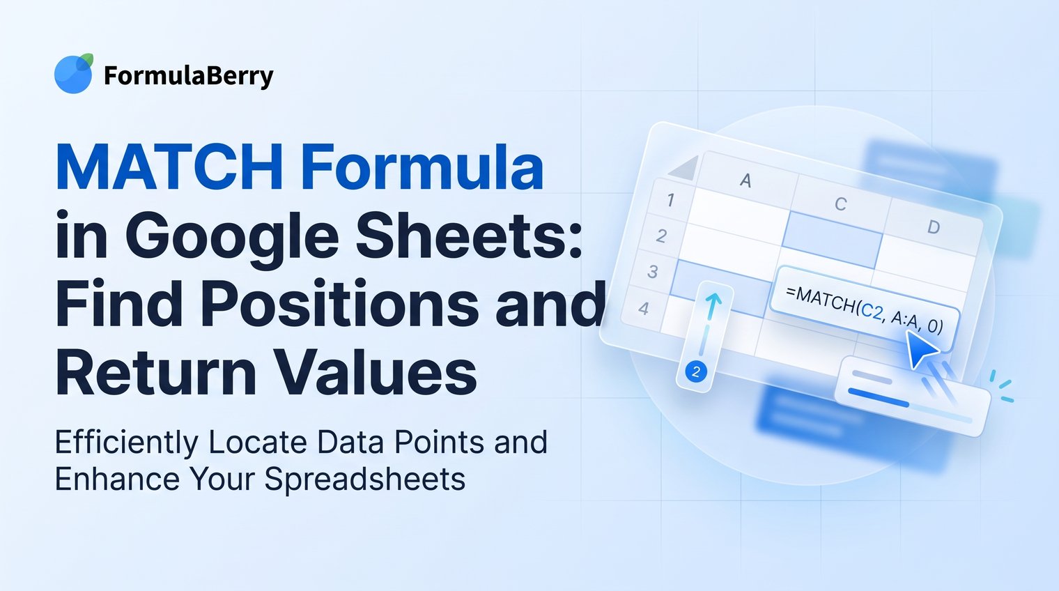
A lookup can appear to work while quietly returning the wrong row. That is why understanding MATCH matters: it tells Google Sheets exactly where an item sits in a list, and it becomes the engine behind flexible INDEX-MATCH lookups.

Whether you are finding a product price, checking two customer lists for overlap, or pulling a value from a monthly report, MATCH gives you a reliable way to locate the right position first.

What MATCH does in Google Sheets

MATCH finds the relative position of an item within a one-dimensional range. It does not return the item itself or a related value from another column. Instead, it returns a number that tells you where the match appears in the range you searched.

The basic syntax is:

=MATCH(search_key, range, [search_type])

For example, if "Notebook" is the fourth item in A2:A10, MATCH returns 4. That result is relative to the selected range, not the worksheet's row numbers. For more ways to work with row positions and references, see Google Sheets ROW Formula: Number Rows and Build References.

MATCH is useful on its own when you only need a position. More often, it supplies the row or column number that INDEX needs to return a related value.

Set up the MATCH formula with an exact match

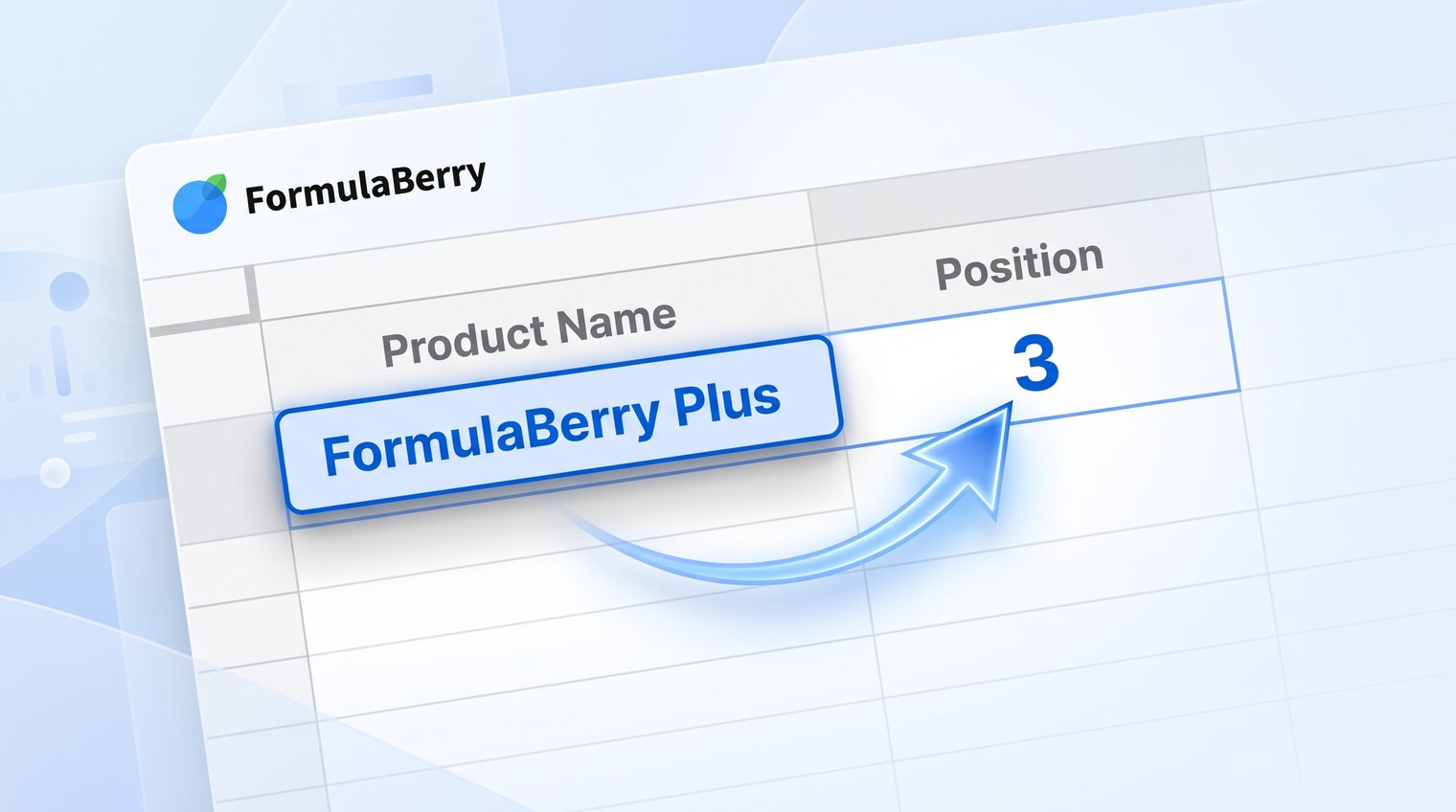
Start with a simple list. Put product names in A2:A10, and type the name you want to find in E2. To find that product's position in the list, enter:

=MATCH(E2,A2:A10,0)

This is the best default pattern for names, order IDs, customer emails, SKUs, and other labels where you need a precise match.

• E2 is the search key: the value you want to locate.
• A2:A10 is the range to search. MATCH works with one row or one column at a time.
• 0 requests an exact match.

Do not omit the final argument when looking up text or identifiers. Using 0 makes your intention clear and prevents Google Sheets from using approximate-match behavior.

Read the result correctly

If the formula returns 3, the matching value is the third cell inside A2:A10. It does not mean the item is on worksheet row 3.

Because this range starts at row 2, a result of 3 points to A4: A2 is position 1, A3 is position 2, and A4 is position 3. This distinction is important when you later feed the MATCH result into INDEX.

Choose the right MATCH search type

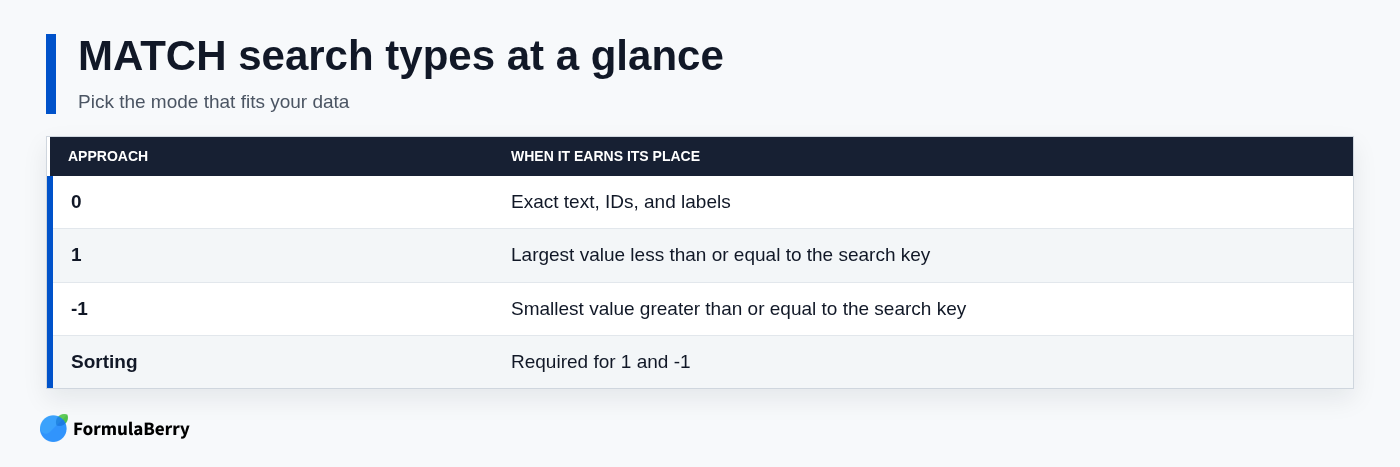
The third MATCH argument controls how Google Sheets searches. For everyday spreadsheet lookups, use 0. It finds an exact value and works regardless of the list's order.

Search type	What it returns	When to use it
0	An exact match	Names, IDs, SKUs, email addresses, and labels
1	The largest value less than or equal to the search key	Sorted numeric ranges in ascending order
-1	The smallest value greater than or equal to the search key	Sorted numeric ranges in descending order

Use 1 for threshold-style data such as tax brackets, discount tiers, or commission bands, but only when the lookup range is sorted from smallest to largest. Use -1 only when the range is sorted from largest to smallest.

A common mistake is using approximate MATCH on an unsorted list. Google Sheets may return a position, but it may not be the one you expect. For labels and identifiers, exact match with 0 is the safer choice.

Return a value with INDEX-MATCH in Google Sheets

MATCH becomes far more useful when paired with INDEX. MATCH identifies the row position, and INDEX returns the value from that same relative position in another column.

Suppose product names are in A2:A10, their prices are in C2:C10, and the product you want is entered in E2. Use:

=INDEX(C2:C10,MATCH(E2,A2:A10,0))

If E2 contains "Notebook," MATCH finds its position in the product list. INDEX then uses that position to return the matching price from column C.

The lookup range and return range do not need to be adjacent. They do need to align row by row. If A2:A10 contains nine products, C2:C10 must contain the corresponding nine prices in the same order.

Break down the INDEX-MATCH formula

For a single return column, the relevant INDEX pattern is:

=INDEX(reference, row)

In the earlier example, C2:C10 is the reference, and MATCH(E2,A2:A10,0) supplies the row number. If MATCH returns 4, INDEX returns the fourth value from C2:C10.

This is why INDEX-MATCH is more flexible than many basic lookups. You can search in one column and return data from a column to its left or right. The column order does not control whether the formula works.

Use a two-way lookup with INDEX-MATCH-MATCH

A two-way lookup retrieves a value from the intersection of a row label and a column header. This is useful for sales reports, staffing schedules, budgets, and any matrix where categories run down the left and periods or measures run across the top.

Imagine products in A2:A10, month headers in B1:E1, and the sales values in B2:E10. If the product is entered in H2 and the month is entered in H3, use:

=INDEX(B2:E10,MATCH(H2,A2:A10,0),MATCH(H3,B1:E1,0))

The first MATCH finds the correct row. The second MATCH finds the correct column. INDEX uses both positions to return the value at their intersection.

Example: find a monthly sales figure

Suppose A2:A10 contains employee names, B1:E1 contains Jan through Apr, and B2:E10 contains each employee's sales totals. Enter an employee name in H2 and a month in H3. The formula returns that employee's sales figure for the selected month. If you need to total the returned figures or related ranges, see Google Sheets SUM Formula: Add Cells, Ranges, and Conditions.

Keep the ranges carefully aligned. The INDEX array, B2:E10, excludes both headers. The first MATCH searches row labels only, A2:A10. The second MATCH searches column headers only, B1:E1.

Including headers inside the INDEX array is a frequent source of off-by-one results. Match the data area to the data area, and match each label range to its own direction.

Compare two columns and flag duplicates with MATCH

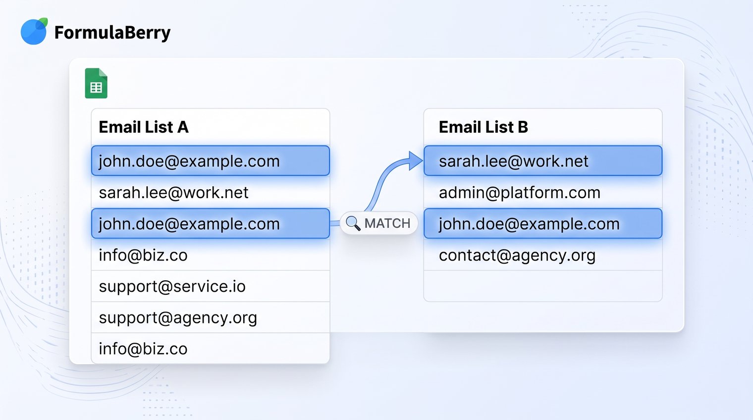
MATCH also makes it easy to compare two lists in Google Sheets. For example, you may have one list of newsletter subscribers in column A and a second export from another platform in column B. You can check whether each value in column A appears anywhere in column B.

In C2, enter:

=IF(ISNUMBER(MATCH(A2,$B$2:$B$100,0)),"Found","Missing")

Then fill the formula down. MATCH returns a position when it finds A2 in the second list, and ISNUMBER converts that position into TRUE. If it cannot find a match, MATCH returns #N/A and the formula displays "Missing."

The dollar signs in $B$2:$B$100 matter. They lock the comparison range so it stays fixed as you copy the formula down column C. Without absolute references, the range would shift one row at a time and produce unreliable results.

This method works well when you need to compare two columns in Google Sheets for duplicates or compare lists for shared customer IDs, invoice numbers, email addresses, or product codes.

Highlight matches with conditional formatting

To visually highlight values in column A that also occur in column B, select the cells you want to format in column A, such as A2:A100. Then create a conditional formatting rule using this custom formula:

=ISNUMBER(MATCH(A2,$B$2:$B$100,0))

Choose a fill color and save the rule. Google Sheets will highlight each value in column A that appears in the comparison list.

This checks for matches across two separate lists. It is not the same as finding duplicate entries within column A itself. For within-column duplicates, the formula needs to count repeats in the same range rather than compare against column B.

Handle #N/A and other common MATCH errors

A #N/A result usually means Google Sheets did not find an exact match. It does not automatically mean your formula is broken. First, confirm that the value in the search cell actually appears in the lookup range.

If the item should match but does not, check these common causes:

• Hidden spaces: "ACME-100" and "ACME-100 " are different values. Clean imported data with TRIM when necessary.
• Text versus numbers: A number stored as text may not match a numeric value that looks identical. Check formatting and imports carefully.
• Wrong search type: Use 0 when you expect an exact match.
• Misaligned INDEX-MATCH ranges: The lookup and return ranges should cover corresponding rows.
• Incorrect cell references: Verify that your search key points to the intended input cell.

When a missing value is expected, wrap the lookup in IFNA so the sheet stays readable:

=IFNA(INDEX(C2:C10,MATCH(E2,A2:A10,0)),"Not found")

This formula returns the price when the product exists and displays "Not found" when it does not. Use IFNA for expected lookup misses; it is better than hiding every possible formula error with a broad error handler.

Decide between INDEX-MATCH, VLOOKUP, and XLOOKUP

The best lookup formula depends on the shape of your data and the result you need.

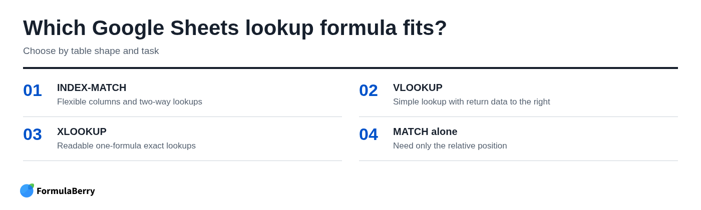
INDEX-MATCH is a strong choice when the return column may move, when you need to look left, or when you need a two-way lookup. Its structure is also portable: once you understand how MATCH supplies positions, you can reuse the pattern in many reports.

VLOOKUP is straightforward for a simple table where the lookup column is on the left and the return data is to the right. It can be quick to write, but inserting or rearranging columns can make its column-number argument harder to maintain.

XLOOKUP is a readable modern alternative for one-directional exact lookups. It separates the lookup range from the return range, which removes VLOOKUP's leftmost-column limitation. INDEX-MATCH remains especially useful for two-way lookups and for spreadsheets where you want a long-standing, familiar formula pattern.

Use MATCH alone when the position itself is the answer, such as determining a rank in a fixed list or locating the column number for a later calculation.

Use MATCH confidently in your next lookup

For most everyday Google Sheets lookups, start with MATCH(...,0). Use MATCH by itself when you need a relative position, or place it inside INDEX when you need to return related data from another row or column.

Build and test the formula on a small sample first. Confirm that the search range, return range, and headers line up before copying it across a larger report. That small check prevents most lookup errors.

If you need help generating, explaining, or fixing an Excel or Google Sheets lookup formula, FormulaBerry can turn a plain-language request into a formula you can use and understand.