A growth Excel formula looks simple until the number is used in a budget, sales report, or board update. Comparing the wrong periods, dividing by zero, or adding monthly percentages can turn a reasonable-looking result into a misleading one.

The right formula depends on the story you need the spreadsheet to tell. Are you measuring change from last month, comparing this March with last March, measuring total change since launch, or finding an annualized rate across several years? Those are different calculations, even when they all produce percentages.

Choose the right growth calculation before you write a formula

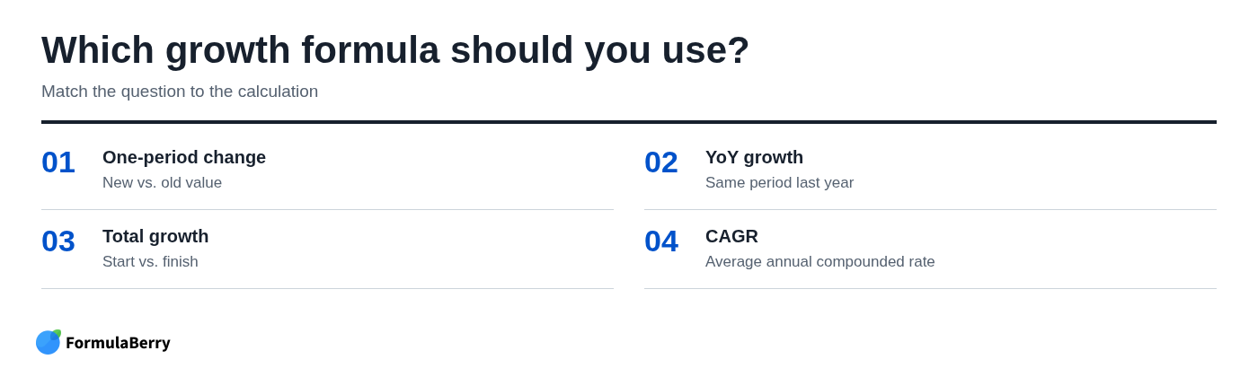
Most growth calculations fall into four categories. Choosing among them first prevents a common spreadsheet mistake: applying one formula accurately to the wrong business question.

• Period-over-period percentage change compares a new value with the immediately preceding or otherwise selected old value.
• Year-over-year (YoY) growth compares the same month, quarter, or reporting period with that period one year earlier.
• Total growth compares a starting value with an ending value across the entire period.
• Compound annual growth rate (CAGR) turns total growth into a constant annual compounded rate.

The core rule is straightforward: every percentage growth calculation needs a baseline, usually the old or beginning value. CAGR also needs the number of compounding periods. If your baseline is zero, blank, or negative, you need to stop and decide how the result should be reported before copying a formula down the sheet.

Quick start: the formulas most readers need

For ordinary percentage growth, use either of these equivalent formulas:

• Growth rate: =(New-Old)/Old
• Equivalent shorthand: =New/Old-1
• CAGR: =(Ending/Beginning)^(1/Years)-1

In Excel, format the result cell as a percentage. Do not multiply the formula by 100 and then apply Percentage formatting, or a true 12% result will display as 1,200%.

Calculate percentage growth in Excel

The standard growth Excel formula measures the change between two values relative to the original value. It answers questions such as, "How much did sales increase from last quarter to this quarter?" or, "What was the percentage change in expenses from January to February?"

Suppose prior-period sales are in cell B2 and current-period sales are in C2. If sales rose from $8,000 to $9,200, the increase is $1,200. Relative to the $8,000 starting point, that is 15% growth.

Use the standard growth formula: =(New Value-Old Value)/Old Value

Enter this formula in a growth column:

=($C2-$B2)/$B2

Or use the shorter version:

=C2/B2-1

Both return the same result. With B2 equal to 8,000 and C2 equal to 9,200, Excel returns 0.15, which becomes 15% when formatted as a percentage. A positive value indicates growth; a negative value indicates a decline.

For a row-by-row report, normally leave the row numbers relative so Excel changes them during fill-down. You may lock columns with dollar signs, as in $C2 and $B2, if the formula will be copied across a wider report and those source columns must stay fixed.

Format the result as a percentage

Select the formula cells, then choose Home > Number > Percent Style. Use the Increase Decimal or Decrease Decimal buttons to show the precision the report needs. For most sales dashboards, one decimal place is enough; for financial modeling, two may be more appropriate.

A frequent error is writing =(C2/B2-1)*100 and then applying Percent Style. That double-converts the answer. Either return the decimal result and format it as a percentage, or multiply by 100 only when you intend to display a plain number without percentage formatting.

FormulaBerry

If you know what the worksheet should calculate but are unsure how to express it in Excel syntax, FormulaBerry can generate a formula from a plain-language request. For example: "Calculate percentage sales growth using prior sales in B2 and current sales in C2, and return N/A when prior sales are blank or zero."

It is especially useful when your real worksheet has nonstandard columns, mixed conditions, or a formula you need explained before using. FormulaBerry generates, explains, and helps correct Excel and Google Sheets formulas. Its Excel formula generator can help with the syntax, but you still need to check whether your periods, source values, and business definition are actually comparable.

Build a fill-down sales growth formula for a table

A recurring sales report usually needs more than one comparison. The goal is to enter a formula once, fill it down, and let Excel adjust the references for every new month or quarter.

Imagine monthly sales in B3:B14, with January in B3 and December in B14. Put the growth result in column C.

Compare each row with the previous row

In C4, enter:

=B4/B3-1

Then fill the formula down through the remaining rows. For February, Excel compares February sales in B4 with January sales in B3. In the next row, it automatically becomes =B5/B4-1, comparing March with February.

Leave C3 blank or label it N/A. January has no prior month in this example, so a month-over-month calculation is not available. Entering zero would wrongly imply that January experienced no change rather than that no comparison exists.

Compare a fixed baseline with every later period

Sometimes you want every month measured against the same starting point, such as January sales. In C4, use:

=B4/$B$3-1

The dollar signs make B3 an absolute reference. When you fill the formula down, the current-month reference changes from B4 to B5, B6, and so on, but the January baseline remains B3.

This is total growth from baseline, not month-over-month growth. A May result of 30% means May sales are 30% above January, even if sales fell compared with April. Label the column clearly so readers do not confuse the two measures.

Calculate year-over-year growth in Excel

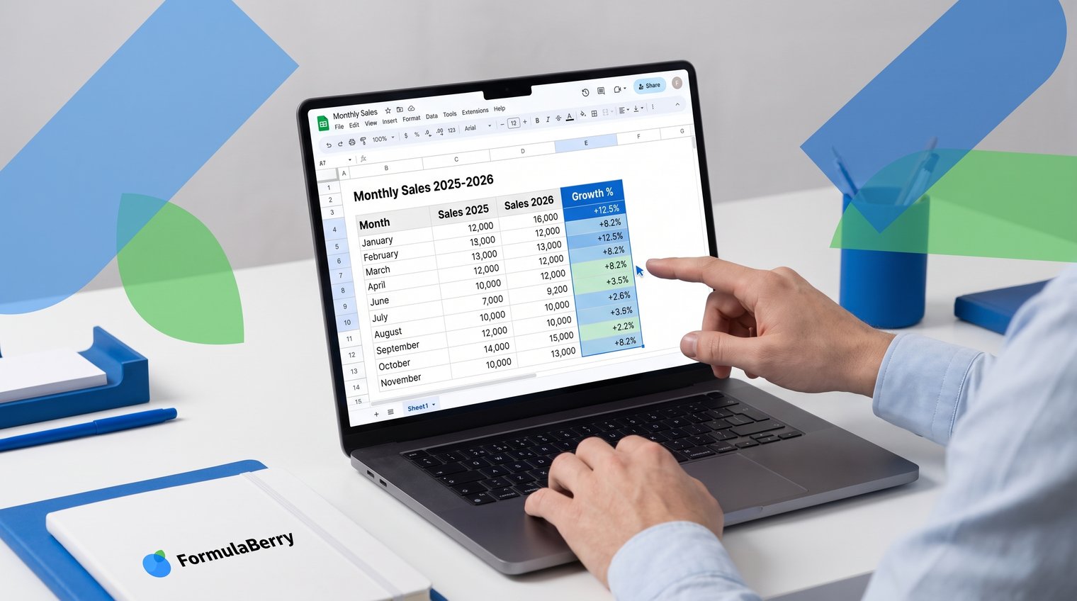
Year-over-year growth compares like for like: January this year against January last year, Q2 this year against Q2 last year, or the current fiscal period against the matching prior fiscal period. This matters because month-over-month numbers can be heavily affected by seasonality.

A retailer may see December sales far above November sales every year. That does not necessarily signal exceptional growth. Comparing December with the prior December is usually more meaningful.

Use a simple YoY formula when both periods are side by side

If B2 contains sales for March last year and C2 contains sales for March this year, use:

=C2/B2-1

For example, if March 2025 sales were $40,000 and March 2026 sales were $46,000, the formula returns 15%. Format the cell as a percentage and label it something specific, such as March YoY Growth.

Calculate YoY% in a monthly data set

In a consistently ordered monthly series, the matching month from the prior year is often 12 rows above. If the current month is in B14 and the matching month last year is in B2, use:

=B14/B2-1

This approach works only when every month is present, data is sorted correctly, and each row represents the same reporting definition. If months are missing, the sheet combines multiple regions, or the data is not in a clean monthly sequence, use a lookup formula or PivotTable instead of relying on a fixed 12-row offset.

Handle zero, blank, and negative starting values correctly

The formula may be short, but denominator problems are not a minor formatting issue. They affect whether a growth percentage is meaningful at all. A good report distinguishes "not available" from an actual 0% result.

When the old value is zero or blank

Percentage growth is undefined when the old value is zero because the formula divides by zero. A blank starting cell should also not be treated as a valid baseline.

Use this formula when B2 is the old value and C2 is the new value:

=IF(OR(B2=0,B2=""),"N/A",C2/B2-1)

This returns N/A rather than an error or a misleading zero. Avoid using IFERROR(...,0) as a default. It hides genuine errors and tells readers that there was no growth when the calculation was actually impossible.

For a new product with zero prior-period sales and $5,000 this period, report the dollar increase, describe it as growth from a zero base, or use a separate new-business flag. Calling it an infinite percentage increase is mathematically defensible but rarely useful in a business report.

When the starting value is negative

Conventional percentage growth becomes counterintuitive when the baseline is negative. Consider a business moving from a $100 loss to a $50 profit. The arithmetic expression =(50-(-100))/-100 returns -150%, even though operating performance clearly improved.

Do not casually describe that result as "-150% growth." Instead, report the absolute change of $150 and use an operating label such as "moved from a loss of $100 to a profit of $50." The same caution applies to comparisons between two negative values. Percentage change can be calculated, but it may not communicate the business reality honestly.

Calculate total growth across multiple periods

Total growth measures the change from the first value to the final value, regardless of how volatile the path was in between. It is the right measure when you need to answer, "How much larger is the business now than it was at the start?"

Use:

=Ending/Beginning-1

If revenue increased from $100,000 to $160,000 over three years, total growth is =160000/100000-1, or 60%. This does not mean revenue grew 20% each year. For an annualized answer, use CAGR, covered later.

Why growth percentages cannot usually be added

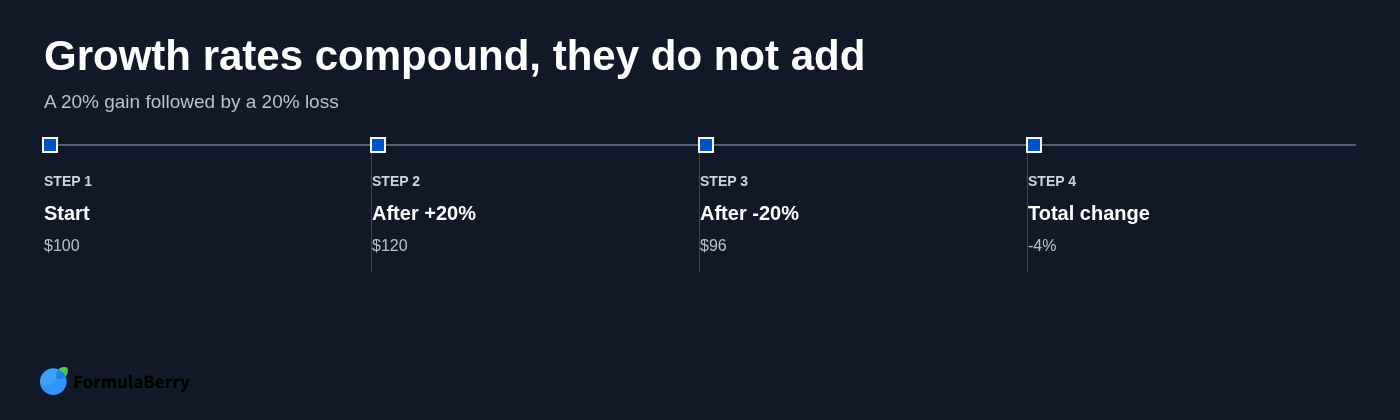
Percent changes compound because each change uses a different base. A 20% gain followed by a 20% loss does not bring you back to where you started.

Starting with $100, a 20% gain produces $120. A subsequent 20% loss applies to $120, leaving $96. The total change is -4%, not 0%.

To calculate total growth safely, compare the first and final values directly. If you must chain known periodic rates, multiply growth factors instead: (1+Rate1)*(1+Rate2)-1.

Use the CAGR formula in Excel for average annual growth

CAGR is the constant annual compounded rate that would turn a beginning value into an ending value over a stated number of years. It is useful for multi-year revenue, customer, market, and investment comparisons because it puts different time spans on an annual basis.

CAGR smooths the path between the start and finish. It does not show actual year-to-year volatility, and it is not the arithmetic average of annual growth percentages.

Write the direct CAGR formula

The direct formula is:

=(Ending Value/Beginning Value)^(1/Number of Years)-1

If B2 contains the beginning value, C2 the ending value, and D2 the number of years, enter:

=($C$2/$B$2)^(1/$D$2)-1

Suppose revenue grew from $100,000 to $172,800 over three years. The CAGR is 20%, because $100,000 multiplied by 1.20 three times equals $172,800.

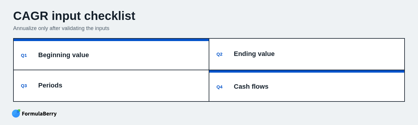
Use the number of intervals, not merely the number of data points. If you have values for the end of 2023, 2024, 2025, and 2026, there are four observations but only three annual intervals between the first and last value.

Use RRI as an alternative CAGR formula

Excel's RRI function calculates the equivalent periodic interest rate:

=RRI(Years,Beginning Value,Ending Value)

Using the same cells, write:

=RRI(D2,B2,C2)

RRI can be easier to read once you know the argument order: number of periods first, present value second, future value third. The direct CAGR formula remains useful because it is transparent and portable across spreadsheet environments.

Count CAGR periods accurately when dates are irregular

A rounded year count can materially distort annualized growth when the start and end dates do not line up exactly. This comes up with fiscal-year reporting, acquisitions, product launches, and data measured on arbitrary dates.

If a value starts on March 15 and ends on November 30 two years later, calling the span "two years" is an approximation. Use the actual time period when accuracy matters.

Calculate fractional years with YEARFRAC

With the beginning value in B2, ending value in C2, start date in D2, and end date in E2, use:

=(C2/B2)^(1/YEARFRAC(D2,E2))-1

YEARFRAC returns the fraction of a year between two dates. By default, Excel uses a standard day-count approach that is generally practical for ordinary business reporting. If you are working with a financial convention that requires a specific basis, review the optional YEARFRAC basis argument and apply the convention used in your organization.

For example, a worksheet can include a start date of March 15, 2023, an end date of November 30, 2025, a beginning value of $250,000, and an ending value of $340,000. Calculate the period length with =YEARFRAC(D2,E2), then use that result in the CAGR formula. This is more defensible than manually typing 2 or 3 years.

Use XIRR when you have multiple cash flows

CAGR is appropriate when you have one beginning value and one ending value. If an investment, project, or account includes deposits, withdrawals, or other uneven cash flows during the period, XIRR is generally more appropriate.

The conceptual formula is:

=XIRR(values,dates)

XIRR uses a range of cash-flow amounts and their corresponding dates to calculate an annualized return. It is not a drop-in replacement for sales growth. Use it for cash-flow-based return analysis, not for ordinary revenue reporting.

Compare growth formulas by business question

Use the question being asked to select the formula, rather than choosing the formula that happens to be familiar.

Business question	Best calculation	Excel formula pattern
How did this period change from the prior period?	Percentage change	=New/Old-1
How did this month compare with last month?	Month-over-month growth	=CurrentMonth/PriorMonth-1
How did this month compare with the same month last year?	YoY growth	=CurrentYear/PriorYear-1
How much did we grow from the start to the finish?	Total growth	=Ending/Beginning-1
What annual compounded rate connects start and finish?	CAGR	=(Ending/Beginning)^(1/Years)-1
What constant rate is needed to reach a target?	Rate-based model	=RATE(nper,0,-pv,fv)

Use the RATE formula for a fixed-rate growth model

The RATE function is useful for modeling a constant periodic rate needed to grow from a present value to a future value:

=RATE(nper,0,-pv,fv)

For example, if a business wants to grow from $100,000 to $150,000 over three years with no interim payments, RATE can calculate the implied annual rate. The present value and future value need opposite signs under Excel's cash-flow convention, which is why the present value is commonly entered as -pv.

RATE is a planning or modeling tool. It differs from measuring observed historical growth, where you already know the actual beginning and ending values and should usually use total growth or CAGR.

Use a growth formula to project a future value

Once you have a growth-rate assumption, a simple future-value formula in Excel is:

=CurrentValue*(1+GrowthRate)^Periods

If current sales are $120,000, the assumed annual growth rate is 8%, and you want a three-year scenario, use =120000*(1+8%)^3. The projected result is approximately $151,174.

That number is a scenario based on an assumption, not evidence of actual future growth. Keep assumptions visible in separate labeled cells so reviewers can change them and see the effect.

Create a reusable growth calculator in Excel

A reusable calculator reduces formula drift in recurring reports. Set up labeled input columns rather than scattering hard-coded numbers through formulas.

A practical layout includes a date or period, prior sales, current sales, calculated growth, growth type, and an error-status field. The growth type can distinguish month-over-month, YoY, baseline growth, or CAGR so a reader understands the comparison without reverse-engineering the formula.

Use Excel Tables and structured references

Convert your source range to an Excel Table with Ctrl+T. Tables automatically expand as new records are added, and their formulas use readable column names instead of cell addresses.

For columns named Prior Sales and Current Sales, use:

=IF(OR([@[Prior Sales]]=0,[@[Prior Sales]]=""),"N/A",[@[Current Sales]]/[@[Prior Sales]]-1)

Excel fills the formula down the table and applies it to new rows as they are added. Structured references make the logic easier to audit because the formula states what it is comparing.

Add conditional formatting without hiding the numbers

Conditional formatting can make a growth column faster to scan. Use clear positive and negative indicators, but keep the actual percentages visible. A green cell with 3% growth and a green cell with 60% growth do not carry the same business significance.

Set sensible thresholds for the report's context. A 5% sales decline may be material in one business and normal variation in another. As covered in the section on zero, blank, and negative values, color also cannot solve an invalid or misleading denominator.

Audit your growth results before sharing them

Before sending a growth report, check five things:

• Are the periods genuinely comparable, especially for YoY calculations?
• Is the denominator the correct old, beginning, or prior-period value?
• Are formula results formatted as percentages without multiplying by 100 twice?
• Does the first row correctly show blank or N/A when no prior comparison exists?
• Does total growth reconcile to the first and final values?

Also inspect unusually large results. They often come from small baselines, missing data, a shifted reference, or a zero value that was hidden by an error-handling formula. A formula explanation tool can help you understand unfamiliar syntax, but it cannot verify the business definition or repair incorrect source data for you.

Apply the formula that matches the growth story

Use percentage change when comparing two comparable values. Use YoY growth when seasonal patterns make same-period annual comparisons more useful. Use total growth to compare the start and finish, and use CAGR when you need that start-to-end change expressed as an annual compounded rate.

The formula is only half the work. A defensible growth number also depends on the right baseline, matched periods, and honest handling of zeros and negative values. If you need help generating, explaining, or correcting a worksheet-specific Excel or Google Sheets formula, FormulaBerry can translate the calculation you need into a usable formula.