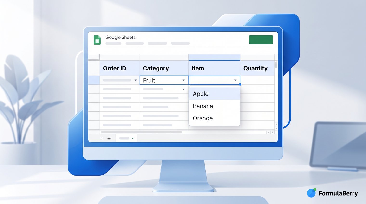
A Google Sheets dependent dropdown list makes the options in one dropdown change based on what someone selects in another. For example, choosing Fruit in a Category column can make the next dropdown show Apple, Banana, and Orange, while choosing Vegetable shows Carrot, Broccoli, and Spinach instead.

This is one of the simplest ways to make order forms, budgets, request trackers, and reporting sheets harder to break. The key is setting up your source data carefully, then connecting the second dropdown to the first with a named range and INDIRECT.

What Is a Dependent Dropdown List in Google Sheets?

A dependent dropdown is a child dropdown whose available choices are controlled by a parent dropdown. The first selection determines which list appears in the second field.

Imagine an order form with Category in column A and Item in column B. If a user selects Fruit in A2, B2 should offer fruit only. If they select Vegetable, B2 should switch to vegetable options. That is different from two independent dropdowns, where both fields always display the same fixed list regardless of the other selection.

Dependent dropdowns reduce invalid entries and make long lists easier to use. Rather than asking someone to scan 100 products, you first narrow the choice to a sensible category.

Set Up the Source Lists on a Separate Sheet

Start by putting your validation lists on a separate tab, such as Lists. This keeps your form clean, makes future edits easier, and reduces the chance that someone accidentally overwrites the source data.

For the standard named-range method, use one column for each parent category. Put the category name at the top of the column and place its child options below it.

Lists!A	Lists!B
Fruit	Vegetable
Apple	Carrot
Banana	Broccoli
Orange	Spinach

You also need a small range containing the parent categories themselves, such as Lists!A1:B1. That range will power the first dropdown in your form.

Keeping lists separate is more than a tidy-sheet preference. It gives you one reliable place to add products, remove discontinued options, or update department names without rebuilding your form.

Use Valid Range Names for Each Category

Named ranges are the link between the parent selection and its matching child list. When someone chooses Fruit, Google Sheets will use that text to locate a named range called Fruit.

Create a named range for each group of child options. In the example above, select Lists!A2:A4 and name it Fruit. Then select Lists!B2:B4 and name it Vegetable.

Range names need to follow a few practical rules:

• Do not use spaces or special characters.
• Use underscores for multi-word names, such as Home_Office.
• Make the range name match the parent dropdown value exactly, unless you deliberately transform the value with a formula.
• Name only the actual options, not a large block of empty cells.

To create one, select the child list, then use Data > Named ranges. Enter the range name in the sidebar and confirm the selected range is correct.

Create the First Dropdown for the Parent Category

The first dropdown should contain your parent categories, such as Fruit and Vegetable. On your form sheet, select the cells where users will choose a category, for example A2:A100.

Then open Data > Data validation, choose Dropdown (from a range), and enter the range containing your category headers. In this example, use:

Lists!A1:B1

Apply the rule to every row you expect people to use. Setting validation for A2:A100 at once is much faster than rebuilding the dropdown each time you add a row.

If the form is likely to grow, leave a reasonable buffer of extra rows. You can always extend the rule later, but it is better to avoid discovering that row 51 accepts unvalidated free text while the first 50 rows do not.

Create the Dependent Dropdown with INDIRECT

The child dropdown uses INDIRECT to convert the selected parent text into a reference to its named range. If A2 contains Fruit, =INDIRECT(A2) resolves to the named range Fruit.

Select the child cells, such as B2:B100, and create another data validation rule. Choose Dropdown (from a range), then enter:

=INDIRECT(A2)

The formula belongs in the validation rule's range field, not directly in B2 as a worksheet formula. B2 remains a dropdown cell where the user makes a selection.

This only works when the text selected in A2 corresponds to a valid named range. If A2 says Fruit, a range named Fruit must exist. A spelling mismatch, trailing space, or different naming style will break the dependency.

Make the Formula Work When Categories Have Spaces

=INDIRECT(A2) fails when your displayed category includes spaces but your named range cannot. For instance, a dropdown value of Home Office cannot directly point to a named range with the same space-separated name.

The usual fix is to display a friendly label in the form but replace spaces with underscores before calling the named range:

=INDIRECT(SUBSTITUTE(A2," ","_"))

With that setup, the parent dropdown can display Home Office, while the matching named range is Home_Office. The formula turns the selected label into the valid range name Google Sheets expects.

You can use the same idea for other deliberate naming differences, but do not make the system unnecessarily clever. Consistent labels and consistent named ranges are easier for the next person maintaining the sheet to understand.

Apply Dependent Dropdowns to Multiple Rows Without Breaking References

For a row-by-row form, each child dropdown should depend on the parent cell in the same row. That means B2 should use A2, B3 should use A3, and so on.

A relative reference is what makes this work. Use =INDIRECT(A2) in the validation rule for the first row, then copy or fill that validation down. Google Sheets should adjust the row relationship as the rule moves down.

By contrast, =INDIRECT($A$2) locks every child dropdown to A2. That is useful only when every row should use one shared category selector, such as a report controlled by a single category choice at the top of the sheet.

Data validation behavior can vary depending on how you copied the cells and how the original rule was applied. After filling down, test a few rows: choose Fruit in A3 and Vegetable in A4, then confirm B3 and B4 show different lists. If they do not, copy the correctly configured validation from the first row into the remaining child cells.

Use a Dynamic Source List When Options Change Frequently

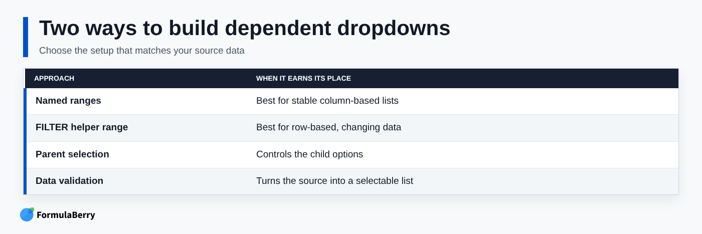
Named ranges are ideal for stable, column-based lists. But if your source data is stored as records in rows and changes often, a FILTER helper range can be easier to maintain.

Suppose a Products sheet has categories in column A and product names in column B:

Products!A	Products!B
Fruit	Apple
Fruit	Banana
Vegetable	Carrot
Vegetable	Broccoli

In an unused helper area, enter a formula such as:

=FILTER(Products!B2:B,Products!A2:A=A2)

It returns only the products whose category matches the value in A2. The results spill down into the helper area, and the child dropdown can reference that spilled list.

This method is often better when you have many categories, one centralized product table, or options that are regularly added and removed. The tradeoff is that the helper area needs enough room to spill without running into other content.

Troubleshoot a Dependent Dropdown That Is Blank or Shows an Error

A blank dependent dropdown usually means Google Sheets cannot find the range the formula is asking for. Start with the parent value and the named range: they must align exactly.

Check these common causes first:

• The parent value does not match the named range, including capitalization, spacing, or underscores.
• The named range includes blank cells or points to the wrong area of the Lists sheet.
• The parent cell is blank, so INDIRECT has no valid range name to resolve.
• The validation formula references the wrong parent row, such as A2 when the dropdown is in row 8.
• The child cell still contains an item from the previous category.

A quick test is to enter =INDIRECT(A2) in an unused cell. If A2 contains Fruit, the formula should return or spill the items from the Fruit named range. If it produces an error, the issue is with the parent value, named range, or formula - not the dropdown itself. For help creating or fixing a more complex formula, see the Google Sheets formula generator.

Also clear a child selection when its parent category changes. If B2 previously contained Apple and A2 changes from Fruit to Vegetable, Apple is no longer a valid answer. Google Sheets may preserve the old value until you remove it, so build that review step into your workflow.

Start with a Reusable Dependent Dropdown Template Layout

A simple two-sheet layout is enough for many forms. Use a Form sheet for entry and a Lists sheet for your validation sources.

Here is a copy-ready structure:

• Form!A1: Category
• Form!B1: Item
• Form!A2:A100: Parent dropdown from Lists!A1:B1
• Form!B2:B100: Child dropdown using =INDIRECT(A2)
• Lists!A1: Fruit, with Apple, Banana, and Orange below it
• Lists!B1: Vegetable, with Carrot, Broccoli, and Spinach below it
• Named ranges: Fruit for Lists!A2:A4 and Vegetable for Lists!B2:B4

Once the structure works, duplicate the pattern for other paired choices: Department and Team, Region and City, Service Type and Package, or Project and Task. The form does not need a new concept each time; it needs clean source data and predictable names.

Build a More Reliable Google Sheets Form

The reliable sequence is straightforward: organize your source lists, create named ranges for the child options, build the parent dropdown, and use INDIRECT in the child validation rule. Test several category changes before sharing the sheet so you catch naming mismatches and row-reference issues early.

Keep the Lists sheet separate from the form, avoid casual edits to range names, and make multi-word labels follow one naming convention. Those small decisions prevent most dependent dropdown problems.

If you need to adapt the setup for a more complex workbook, FormulaBerry can help generate, explain, or correct a Google Sheets formula from a plain-language description of what you want the sheet to do.