

Missing values invite bad spreadsheet habits. People often eyeball a chart, pick a convenient nearby number, and move on. A linear interpolation formula gives you a better answer: a visible estimate based on the two data points surrounding the gap.
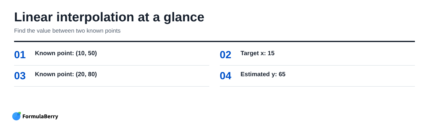
For example, if x = 10 corresponds to y = 50 and x = 20 corresponds to y = 80, the estimated y-value at x = 15 is 65. The target sits halfway between the two x-values, so the estimate sits halfway between the two y-values.
Excel does not have a single built-in INTERPOLATE worksheet function. Instead, you calculate linear interpolation with a short formula. This applies within a known range; estimating beyond the last known point is extrapolation, which carries more risk.
The interpolation result: estimate the missing value between known Excel data points
Interpolation is useful when you have a known relationship in a table but need an estimate for an unlisted input. In the example above, the data points are (10, 50) and (20, 80), and the target is x = 15. Because 15 is exactly halfway from 10 to 20, the linear estimate is 65.
That result assumes the y-value changes at a steady rate between the two surrounding points. It is a practical assumption for many local calculations, including price tiers, calibration readings, conversion factors, and planning estimates, but it is not a guarantee that real-world data always behaves in a straight line.
What interpolation means in Excel
In a spreadsheet, interpolation means estimating a dependent value, usually y, for an input value, usually x, that falls between values already in your data. You are not looking for an exact table match. You are estimating the point between two matches.
Linear interpolation assumes a constant rate of change from the lower point to the upper point. If quantity rises by 10 and price rises by 30, the model assumes that a quantity increase of 5 produces a price increase of 15.
That assumption is reasonable when the two nearby points appear to follow a roughly straight relationship. It is less suitable when prices jump at thresholds, measurements follow a curve, or a business rule determines the answer.
The simplest linear interpolation formula in Excel
The standard linear interpolation formula is:
y = y1 + (x - x1) * (y2 - y1) / (x2 - x1)
In plain language, start with the lower y-value, then add the appropriate share of the change between the two y-values. The share is determined by how far the target x-value sits between x1 and x2.
Suppose column A contains x-values, column B contains y-values, and E2 contains the target x-value. If the two source rows are rows 2 and 3, use:
=B2+(E2-A2)*(B3-B2)/(A3-A2)
Here, A2 is x1, B2 is y1, A3 is x2, B3 is y2, and E2 is the target x. The formula returns the estimated y-value.
How the formula calculates the fraction between two values
The important part is (x-x1)/(x2-x1). It identifies the target's position between the lower and upper x-values.
Using x1 = 10, x = 15, and x2 = 20, the fraction is:
(15-10)/(20-10) = 5/10 = 0.5
The target is 50% of the way from 10 to 20. The y-values rise from 50 to 80, a difference of 30. Half of 30 is 15, so the formula returns 50 + 15, or 65.
How to avoid common cell-reference errors
For one calculation, ordinary relative references are fine. When you want to fill a formula down for several target values, decide which cells should move and which should stay fixed.
If every row has its own pair of bracketing values, relative references are usually correct. If all targets use the same two endpoints, lock those endpoint cells with dollar signs, such as $A$2 and $B$2. A target cell in E2 can remain relative so it changes to E3, E4, and so on as you fill down.
- Make sure x1 and x2 are different. Otherwise, the formula divides by zero.
- Use two points that bracket the target: x1 below the target and x2 above it.
- Keep the lower and upper points paired correctly. Do not use an x-value from one row and a y-value from another.
Worked example: interpolate a price at an unlisted quantity
Consider this illustrative quantity-and-price table. The values are examples only, but the worksheet setup is reproducible.
| Quantity | Price |
|---|---|
| 100 | 240 |
| 200 | 420 |
| 300 | 600 |
A pricing analyst needs an estimate for a quantity of 150. The target sits between 100 and 200, so those are the two rows to use. Enter 150 in E2, then enter this formula in F2:
=B2+(E2-A2)*(B3-B2)/(A3-A2)
The result is 330. Quantity 150 is halfway between 100 and 200, while 330 is halfway between 240 and 420. That is a useful first validation check: with a target at the midpoint, the result should be the midpoint of the two prices under a linear model.
The estimate also falls between the known prices of 240 and 420. If it did not, the most likely causes would be an incorrect cell reference, reversed endpoints, or a target value outside the bracket.
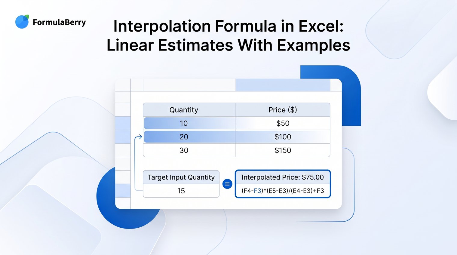
How to interpolate between two values in an Excel table
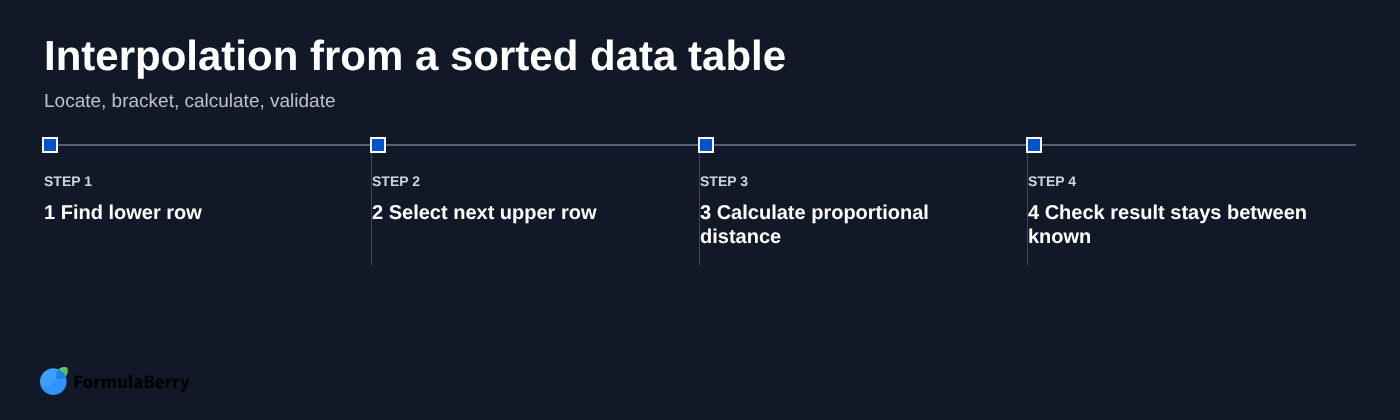
The two-row example is easy because the surrounding values are obvious. In a longer table, the real work is finding the row immediately below the target and the next row above it.
Start by sorting the x-values in ascending order. Then locate the lower bracketing row, select the next row as the upper bracket, and use the same linear interpolation formula. If the target exactly matches an x-value already in the table, return the existing y-value rather than calculating an estimate.
Find the surrounding rows with XLOOKUP
In current Microsoft 365 and newer Excel versions, XLOOKUP can retrieve the values on either side of a target. Assume x-values are in A2:A10, y-values are in B2:B10, and the target is in E2.
One readable approach is to place the surrounding values in helper cells:
| Cell | Formula | Purpose |
|---|---|---|
| G2 | =XLOOKUP(E2,A2:A10,A2:A10,,-1) | Lower x-value |
| H2 | =XLOOKUP(E2,A2:A10,B2:B10,,-1) | Lower y-value |
| G3 | =XLOOKUP(E2,A2:A10,A2:A10,,1) | Upper x-value |
| H3 | =XLOOKUP(E2,A2:A10,B2:B10,,1) | Upper y-value |
In XLOOKUP, match mode -1 finds an exact match or the next smaller item, while match mode 1 finds an exact match or the next larger item. Keep the exact-match lookup separate from the interpolation branch so matching lower and upper rows do not cause division by zero. Use:
=IFERROR(XLOOKUP(E2,A2:A10,B2:B10),IF(OR(E2<=MIN(A2:A10),E2>=MAX(A2:A10)),"Target is outside the interpolation range",H2+(E2-G2)*(H3-H2)/(G3-G2)))
Helper cells are not a weakness. They make the bracket selection easy to inspect, which matters when someone else needs to audit the workbook or troubleshoot a result.
Use MATCH and INDEX in older Excel versions
Older Excel versions do not include XLOOKUP, but MATCH and INDEX handle the same workflow. First check for an exact match with =IFERROR(INDEX(B2:B10,MATCH(E2,A2:A10,0)),"") and use that y-value when one is returned. For interpolation, continue only when the target is strictly between the first and last sorted x-values; use this in G2 to return the position of the lower row:
=IF(OR(E2<=MIN(A2:A10),E2>=MAX(A2:A10)),"Check target range",MATCH(E2,A2:A10,1))
Then retrieve the lower and upper x- and y-values with INDEX:
| Cell | Formula |
|---|---|
| G3 | =INDEX(A2:A10,G2) |
| H3 | =INDEX(B2:B10,G2) |
| G4 | =INDEX(A2:A10,G2+1) |
| H4 | =INDEX(B2:B10,G2+1) |
Use G3 and H3 as the lower point and G4 and H4 as the upper point in the interpolation formula. Approximate MATCH with a match type of 1 depends on ascending sort order. If the x-values are unsorted, it can select the wrong row without making the mistake obvious.
Before-and-after: replace manual estimates with a reusable interpolation setup
A common manual process looks harmless at first: someone receives a quantity that is not on the rate table, checks the nearest rows, estimates the price mentally, and sends an answer. The problem appears when several requests arrive or another person needs to verify how the number was chosen.
In a representative pricing-analysis scenario, an analyst receives a list of quantities missing from a sorted rate table. Instead of calculating each estimate separately, they add a target-quantity column, use lookup logic to identify the lower and upper rows, and fill the interpolation formula down.
The result is not merely faster. Each estimate has visible source inputs, a clear formula, and a checkable assumption: the relationship is treated as linear between nearby table values. That makes the workbook easier to review, update, and hand off.
- Sort the source table before using approximate lookup logic.
- Keep the lower and upper bracket values visible when the table is important enough to audit.
- Use a fill-down formula for repeated requests instead of recreating arithmetic each time.
- Document whether the estimate is linear, especially when it supports a quote, budget, or operational decision.
When linear interpolation is the wrong model
Linear interpolation is a local estimate, not a universal rule. A straight line can be misleading when data curves sharply, changes in steps, or follows an explicit policy rather than a smooth mathematical relationship.
Before relying on the formula, look at a scatter chart and consider the process behind the numbers. A shipping table with hard quantity thresholds may require a direct lookup. A physical measurement may follow a curve. A tax or discount calculation may be determined entirely by bands and rules.
Exponential interpolation for multiplicative growth
If y changes multiplicatively and remains positive, interpolate the natural log of y-values, then convert the result back with EXP. This can be appropriate for compound growth or some decay processes, where equal x-intervals represent proportional rather than absolute changes.
The pattern is:
=EXP(LN(y1)+(x-x1)*(LN(y2)-LN(y1))/(x2-x1))
For cell references, that might be:
=EXP(LN(B2)+(E2-A2)*(LN(B3)-LN(B2))/(A3-A2))
That formula assumes B2 and B3 are positive. More importantly, it is a modeling decision based on how the data behaves, not a more advanced default for every spreadsheet.
Log-linear interpolation when x is on a logarithmic scale
Log-linear interpolation is different because it transforms x, not y. Use it when the spacing of x-values is meaningful on a logarithmic scale, such as ranges that grow by factors rather than fixed increments.
The pattern is:
=y1+(LOG(x)-LOG(x1))*(y2-y1)/(LOG(x2)-LOG(x1))
All x-values involved must be positive. Do not confuse this with exponential interpolation: exponential interpolation transforms y-values, while log-linear interpolation transforms x-values.
Nonlinear curves and multiple variables
Two points cannot reliably describe a complicated curve, and they certainly cannot capture a result driven by several inputs. If output depends on quantity, location, product type, season, and contract terms, a two-point formula may hide more than it explains.
Gather more observations and choose a method that fits the decision. A chart trendline can help with exploratory work, while LINEST regression in Excel or a dedicated business model may be appropriate for higher-stakes calculations. The right question is not, "Which Excel function should I use?" It is, "What relationship do these inputs actually follow?"
How to validate an interpolation formula before relying on it
Interpolation formulas are short enough to look trustworthy even when they reference the wrong cells. A few quick checks catch most problems before the estimate reaches a report or decision-maker.
- Confirm the target x-value falls between the selected lower and upper x-values.
- For lookup-based formulas, confirm the x-column is sorted ascending.
- When the local y-values increase or decrease steadily, verify the result falls between y1 and y2.
- Set the target equal to x1. The formula should return y1.
- Set the target equal to x2. The formula should return y2.
- Check for duplicate x-values, blank source cells, and targets outside the table range.
Duplicate x-values deserve special attention because they can produce division-by-zero errors. Targets outside the source range should be handled deliberately: either return a message, stop the calculation, or use an explicitly approved extrapolation approach. Do not let an approximate lookup silently turn an out-of-range request into a misleading estimate.
Apply interpolation formulas with confidence
Use the core linear interpolation formula when the target lies between two known points and a straight-line change is a reasonable local approximation. For larger tables, add XLOOKUP or MATCH and INDEX logic to find the surrounding rows, then validate the selected bracket and result.
Change the model only when the relationship calls for it. A more complicated formula is not automatically more accurate; it must reflect the way the underlying data behaves.
If you need help generating, explaining, or correcting an Excel or Google Sheets interpolation formula for your table layout, FormulaBerry can turn a plain-language request into a formula you can review and use.