LINEST is Excel's built-in linear regression function. It calculates a least-squares best-fit line and can return the slope, intercept, and a fuller set of regression statistics when you need more than a chart trendline equation.

For a simple model, LINEST helps you estimate an equation in the form y = mx + b: the predicted outcome equals the slope times the input, plus the intercept. It is useful for questions such as whether advertising spend relates to sales, whether production hours affect output, or how a budget category changes over time. For comparisons across periods, you may also need a growth Excel formula.

What the LINEST Excel Formula Does

The LINEST Excel formula fits a straight line to your data using the least-squares method. In practical terms, it finds the line that minimizes the combined squared distance between the observed values and the values predicted by the line.

That is more substantial than simply drawing a trendline on a chart. A chart can display an equation, but LINEST gives you the underlying coefficients and, when requested, statistics that help you judge how well the model fits the data.

In the formula, known_y's are the values you want to predict or explain. Known_x's are the input values that may influence those outcomes. If sales are in one column and ad spend is in another, sales are y and ad spend is x.

LINEST Syntax and Its Four Arguments

The full syntax is:

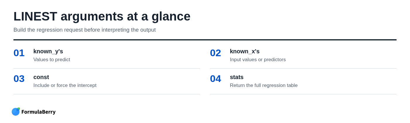
=LINEST(known_y's, [known_x's], [const], [stats])

The square brackets mean an argument is optional. That does not mean the optional choices are unimportant: the const and stats settings can materially change both the model and the size of the returned result.

Argument	What it controls
known_y's	The observed outcome values you want the model to predict, such as sales.
known_x's	The input or predictor values, such as advertising spend, price, or units sold.
const	TRUE estimates an intercept. FALSE forces the intercept to zero.
stats	TRUE returns additional regression statistics. FALSE returns only the coefficients.

If you omit known_x's, Excel assumes a sequence of 1, 2, 3, and so on. That can be useful for a trend across ordered periods, but it is usually clearer to provide the actual x range when one exists.

For most business spreadsheet models, start with const=TRUE. Use stats=FALSE when all you need is the equation, and switch to TRUE when you need to evaluate the fit.

How to Use LINEST for a Simple Linear Regression

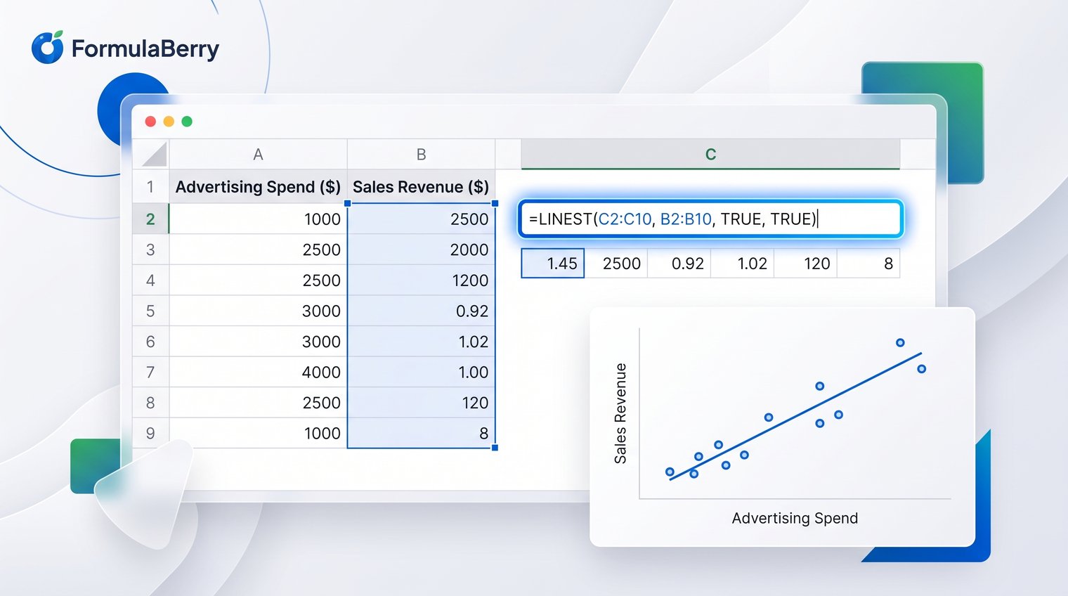
Suppose monthly advertising spend is in cells A2:A11 and monthly sales are in B2:B11. To estimate the relationship between spend and sales, enter:

=LINEST(B2:B11,A2:A11,TRUE,FALSE)

Sales are the y values because they are the outcome being estimated. Advertising spend is the x value because it is the predictor. With one x variable and stats set to FALSE, LINEST returns two values: the slope first and the intercept second.

If the returned slope is 4.2 and the intercept is 1,500, your fitted equation is:

Sales = 4.2 x Ad Spend + 1,500

Interpret units carefully. If ad spend is recorded in dollars, the slope suggests that each additional dollar of spend is associated with an estimated $4.20 increase in sales within this data set. It does not, by itself, prove that spending caused the increase. For related percentage changes and business calculations, see this guide to the Excel percentage formula.

In modern Excel, results that occupy multiple cells typically spill automatically. In older Excel versions, select a two-cell horizontal destination range first, enter the formula, and confirm it with Ctrl+Shift+Enter as an array formula.

How to Read the Full LINEST Results Table

Set the final argument to TRUE when you want more than the equation:

=LINEST(B2:B11,A2:A11,TRUE,TRUE)

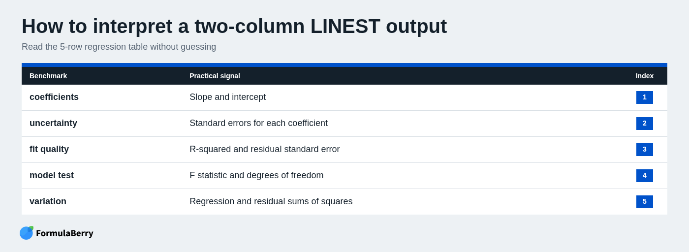
For one predictor, Excel returns a five-row, two-column array. The first row contains the coefficients; the remaining rows provide error, fit, and variation measures. This is where LINEST becomes far more useful than a basic chart label.

Row	First column	Second column
1	Slope	Intercept
2	Standard error of slope	Standard error of intercept
3	R-squared	Standard error of y estimate
4	F statistic	Degrees of freedom
5	Regression sum of squares	Residual sum of squares

Row 1 gives the equation. The slope describes the estimated change in y for a one-unit increase in x, while the intercept is the model's estimated y value when x is zero.

Row 2 addresses coefficient uncertainty. Smaller standard errors, relative to the coefficient values, generally indicate more precise estimates. They are not confidence intervals or prediction intervals, however. A prediction interval concerns the range where a future individual observation might fall, and LINEST does not place that range directly into this table.

Row 3 contains R-squared and the standard error of the y estimate. R-squared indicates the proportion of variation in y explained by the model within this sample. The standard error of y shows the typical size of the residual errors in y units, which is often easier to interpret operationally.

Rows 4 and 5 are more diagnostic. The F statistic evaluates the model as a whole, while degrees of freedom depend on the number of observations and estimated parameters. The two sums of squares divide variation into the amount explained by the regression and the amount left unexplained.

When to Set const to FALSE

Set const to FALSE only when the intercept should genuinely be zero. Doing so forces the model into the form y = mx, meaning that zero input must produce zero output according to the model.

Compare these formulas:

=LINEST(B2:B11,A2:A11,TRUE,FALSE)
=LINEST(B2:B11,A2:A11,FALSE,FALSE)

The first estimates both slope and intercept. The second forces sales to be zero when ad spend is zero. That may be inappropriate because sales can come from repeat customers, organic demand, seasonality, or other channels even with no advertising spend.

A zero intercept can be appropriate when a real-world rule supports it, such as a quantity calculated from a fixed per-unit rate with no baseline amount. Do not choose it merely because the equation looks cleaner. Forcing the line through zero can change the slope substantially and worsen the model's usefulness.

Using LINEST With Multiple X Variables

LINEST can also estimate multiple linear regression when your x values occupy several adjacent columns. For example, if sales are in D2:D20 and the predictors are ad spend, discount rate, and website visits in A2:C20, use:

=LINEST(D2:D20,A2:C20,TRUE,TRUE)

Conceptually, the result fits a model like:

y = m1x1 + m2x2 + m3x3 + b

One detail catches many users: Excel returns the coefficients for x columns in reverse order, followed by the intercept. For A2:C20, the first coefficient corresponds to column C, the next to column B, then column A, followed by the intercept. Label the output cells before sharing results so a coefficient is not assigned to the wrong variable.

Multiple predictors can make a model more useful, but they also make interpretation less casual. Each coefficient represents the estimated relationship with y while holding the other included predictors constant.

LINEST Errors and Results That Do Not Match a Chart Trendline

When LINEST results do not match a chart trendline, check the data selection and intercept setting before assuming Excel is wrong. Most mismatches come from formulas and charts using slightly different assumptions.

• Unequal ranges: The y range and x range must contain the same number of observations.
• Text or errors in the source data: Values stored as text, blanks handled inconsistently, and error cells can affect results or cause formula errors.
• A forced intercept: A trendline may estimate an intercept while LINEST uses const=FALSE, or the reverse.
• Different selected ranges: Confirm that both the chart and LINEST include the same rows.
• Rounded chart labels: Trendline equations shown on a chart are often rounded, so compare the actual cell values rather than the displayed label.

Filtering can add confusion as well. Confirm what data the chart and formula are actually using, particularly in workbooks where rows are hidden, filtered, or copied into helper ranges.

A Practical LINEST Checklist Before You Trust the Model

A correct formula does not automatically produce a useful model. Before using LINEST output in a report, inspect the data and ask whether the relationship makes practical sense.

• Create a scatter plot and look for a roughly linear pattern rather than a clear curve, cluster, or abrupt break.
• Check obvious outliers. One unusual month, campaign, or data-entry error can pull a regression line in a misleading direction.
• Verify that each x value aligns with the correct y value and that the units are consistent.
• Review R-squared alongside the residual error, not as a stand-alone verdict.
• Remember that correlation is not causation. A strong fit may reflect seasonality, a shared trend, or an omitted factor.

A high R-squared can still be unhelpful if the relationship has no sensible business explanation or if prediction errors are too large for the decision at hand. LINEST supplies fit statistics and coefficient uncertainty, but significance and future prediction risk require judgment beyond one number.

Use LINEST When You Need More Than a Trendline Equation

LINEST is the right Excel formula when you need a regression equation plus the evidence behind it. Start by organizing a clean y range and matching x range, decide whether an intercept belongs in the model, and use stats=TRUE when you need to assess coefficients, fit, and residual variation together.

For simple analysis, the slope and intercept may be enough. For a report, forecast, or decision that depends on the result, read the full output rather than relying only on a chart equation.

If you need help building, checking, or translating a LINEST formula into plain English for Excel or Google Sheets, FormulaBerry can generate, explain, and correct spreadsheet formulas from a natural-language request.