A loan payment can look manageable until you ask the more useful question: how much can that payment actually support? The same Excel PV formula can answer that question, or work in reverse to show the lump sum you need today to fund future withdrawals.

The key is treating timing, interest, and cash-flow signs consistently. Excel's PV function returns the value today of regular future payments, but whether that result displays as positive or negative depends on which side of the transaction you are modeling.

The result first: turn future payments into today's value with Excel PV

PV stands for present value: the amount a stream of future payments is worth right now after accounting for interest. If you know the payment, rate, and term of a loan, PV estimates the principal those payments can repay. If you expect to receive regular withdrawals from an investment, it estimates the amount required upfront.

This is not just a finance-class calculation. It is useful when comparing a car loan offer, setting a borrowing limit, planning retirement withdrawals, or determining whether a savings balance can support a future goal.

One detail catches many spreadsheet users: Excel uses opposite signs for money paid and money received. A monthly payment entered as a negative outflow generally produces a positive loan amount. Enter that payment as positive, and Excel returns the same value as a negative number.

What the PV function does in Excel

The Excel PV function calculates the current value of future periodic payments at a specified periodic interest rate. In practical terms, it answers, "What is this series of equal payments worth today?"

Common uses include calculating a loan amount from an affordable payment, valuing an annuity, estimating the starting balance needed for retirement withdrawals, and discounting regular investment cash flows. The important limitation is that payments must be equal and occur at regular intervals.

PV and PMT are related, but they are not the same. PV calculates a starting value, such as a loan principal or initial investment. PMT calculates the recurring payment needed to reach or repay that value. If you know the payment and want the amount financed, use PV. If you know the amount financed and need the payment, use PMT.

PV formula syntax and argument meanings

The PV function syntax is:

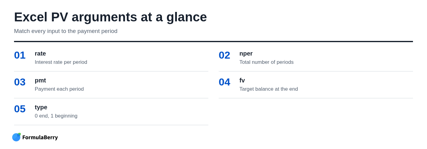
=PV(rate, nper, pmt, [fv], [type])

• rate: Interest rate for each payment period. For monthly payments, use the monthly rate rather than the annual rate.
• nper: Total number of payment periods.
• pmt: Payment made each period. This should remain the same throughout the calculation.
• fv: Optional future value, or balance remaining at the end of the term. If omitted, Excel assumes zero.
• type: Optional timing indicator. Use 0, or omit it, for end-of-period payments; use 1 for beginning-of-period payments.

The rule that matters most is simple: rate and nper must describe the same period. Monthly payments require a monthly rate and a monthly number of periods. Quarterly payments require quarterly inputs.

Before entering the formula: make the time periods consistent

Most incorrect PV results are setup errors, not Excel errors. People often enter an annual rate while using a monthly or quarterly payment count. That mixes units and can produce a result that looks plausible while being materially wrong.

For monthly payments, divide the annual interest rate by 12 and multiply the number of years by 12. For example, a 6% annual rate over five years becomes 6%/12 for rate and 5*12 for nper.

For quarterly payments, divide the annual rate by 4 and multiply years by 4. A three-year arrangement with quarterly payments has 12 periods, not three.

Your payment must follow the same pattern. A monthly PMT belongs with a monthly rate and monthly period count. Do not enter an annual payment into a calculation built around 12 monthly periods.

Example 1: calculate how much you can borrow from a monthly payment

Consider a representative loan-planning situation. A borrower can afford $400 per month, expects a 6% annual interest rate, and wants to repay the loan over five years. What loan principal can those payments support?

Set up the calculation this way:

• Annual rate: 6%
• Monthly rate: 6%/12
• Total months: 5*12
• Monthly payment: -400

The formula is:

=PV(6%/12,5*12,-400)

The result is approximately $20,689.92. The payment is negative because it is cash leaving the borrower's perspective. Excel therefore returns a positive amount for the money received at the beginning: the estimated loan principal.

This is a useful affordability estimate, not a complete loan quote. It excludes origination fees, taxes, insurance, penalties, and rate changes. Still, it gives a practical starting point before you compare lenders or commit to a purchase price.

Why the Excel PV result is negative - and how to control the sign

A negative PV result is often correct. Excel follows a cash-flow convention: money received and money paid must have opposite signs.

Using the same loan example, entering the payment as a positive number gives:

=PV(6%/12,5*12,400)

Excel returns approximately -$20,689.92. It is representing the loan balance as a cash outflow relative to the positive payments you entered. The financial magnitude has not changed; only the viewpoint has.

For a borrowing calculation, many people prefer to enter payments as negative and receive a positive principal amount. For an investment or lender analysis, the opposite convention may make more sense. Pick one viewpoint, label it clearly, and keep every related cash flow consistent. Do not flip signs simply because a result looks unfamiliar.

Example 2: find the lump sum needed today for a savings goal

PV also works for future income planning. Imagine a representative investor who wants to withdraw $1,000 at the end of every year for 10 years. They expect the invested balance to earn 5% annually, and they want the account fully used after the final withdrawal.

The formula is:

=PV(5%,10,-1000,0,0)

The result is approximately $7,721.73. In this case, the future withdrawals are entered as negative because they are payments leaving the investment account. The positive PV result is the amount the investor would need to put aside today, assuming the 5% return and annual withdrawal schedule hold.

This example highlights what PV is really doing: it discounts future money back to a value today. A dollar needed 10 years from now has a lower present value than a dollar needed next year because invested funds have time to earn a return.

When to use FV in a savings calculation

Use PMT when the plan involves equal recurring payments or withdrawals. Use FV when you are working toward one ending balance, balloon payment, or single target amount. For a broader explanation of ending balances and savings targets, see this guide to the FV formula in Excel.

For example, if you need $25,000 in five years and will make no interim deposits, a useful pattern is:

=PV(rate,nper,0,-fv)

If the annual return is 5%, the formula becomes =PV(5%,5,0,-25000). The negative future value produces a positive present investment requirement from the saver's point of view.

Example 3: use the Excel PV formula for quarterly payments

Quarterly arrangements are where period alignment becomes especially important. Suppose an agreement pays $750 at the end of each quarter for three years, with an 8% annual rate.

There are four quarters in a year, so the rate per period is 8% divided by 4, and the number of periods is three years multiplied by 4. The formula is:

=PV(8%/4,3*4,-750,0,0)

This returns approximately $7,942.97. The calculation discounts 12 equal quarterly payments at a 2% quarterly rate.

A common mistake is using 8% as the rate while entering 12 for nper. That treats every quarter as if it had an 8% interest rate, effectively applying the annual rate four times per year. The result will be wrong even though the formula has no error message.

Example 4: account for payments at the beginning of each period

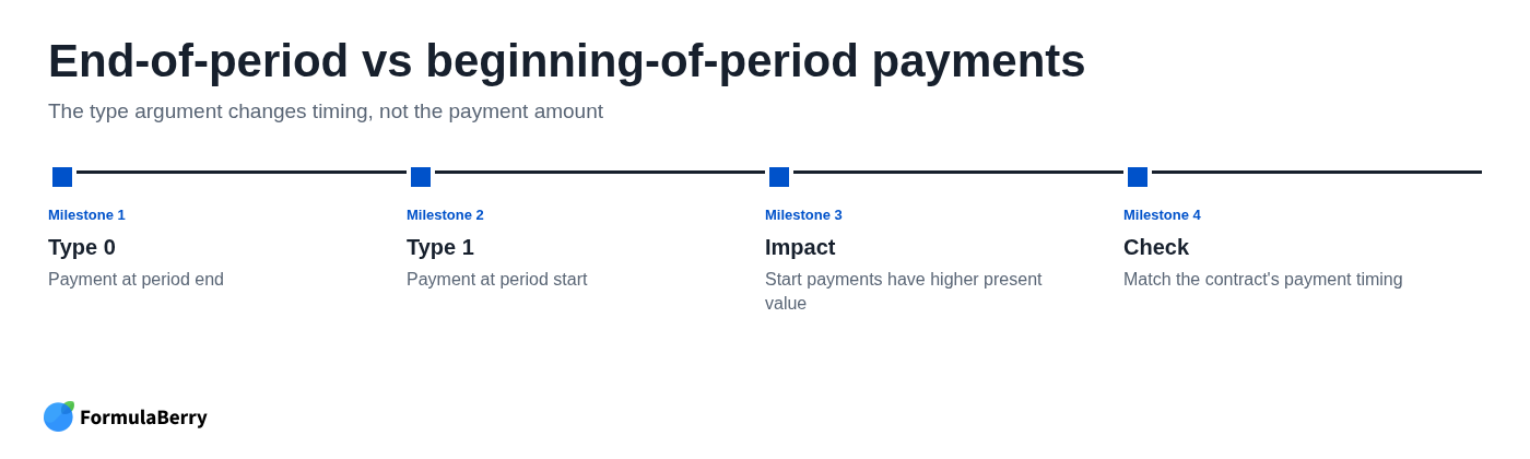
The optional type argument determines when payments occur. Use 0, or leave the argument blank, when payments happen at the end of a period. Use 1 when they happen at the beginning.

Think about a lease or a deposit arrangement. If a payment is due immediately at the start of each month, it has one less month to be discounted than a payment due at the end of that month.

For a representative example with a 6% annual rate, 12 monthly payments of $500, and no ending balance:

=PV(6%/12,12,-500,0,0)

That models payments at month-end. To model the same $500 payments due at the beginning of each month, use:

=PV(6%/12,12,-500,0,1)

The beginning-of-period result is higher because every payment arrives sooner. The payment amount did not change; the timing did. Always check the contract or payment schedule rather than assuming a standard monthly arrangement is automatically end-of-month.

How to calculate present value when payments are different

Excel's PV function is built for equal, regular payments at a constant rate. It is not the right tool when cash flows vary from period to period.

For a small number of uneven payments, discount each cash flow separately and add the results. If a payment occurs in period 3, for example, use:

=cash_flow/(1+rate)^period

If you expect $500 in year 1, $900 in year 2, and $1,200 in year 3 at a 5% annual rate, calculate each amount's present value using periods 1, 2, and 3, then add them with the Excel SUM formula.

For a larger range of regularly spaced but variable cash flows, Excel's NPV function is generally the better fit. For actual payment dates that are irregular, use XNPV. The distinction matters: forcing unequal cash flows into PV can make a neat spreadsheet, but not an accurate financial model. If dates are part of the schedule, this Excel date formula guide can help with date setup and comparisons.

PV formula mistakes to check before trusting the answer

A correct-looking formula can still be based on the wrong assumptions. Before relying on a PV result, check these points:

• Rate and period mismatch: A monthly payment schedule needs a monthly rate and monthly nper value.
• Sign confusion: Payments and the value received should have opposite signs. A negative result is not automatically a mistake.
• Missing type argument: If payments begin immediately, type should usually be 1 rather than the default 0.
• Payment unit mismatch: Do not use an annual payment with monthly periods or a monthly payment with yearly periods.
• Wrong function for the cash-flow pattern: PV assumes equal payments and a fixed periodic rate. It does not directly handle variable-rate loans or irregular payment schedules.

A simple validation habit helps: write the actual schedule in plain language before entering the formula. Label the interest rate as annual, monthly, or quarterly; label the payment frequency; and confirm whether the first payment occurs now or after the first period. Clear labels often reveal mistakes faster than inspecting the formula itself.

A repeatable PV worksheet setup you can use for any scenario

A reusable worksheet makes PV calculations easier to audit and update. Put assumptions in separate input cells rather than burying every number inside one long formula.

Input	Example cell	Purpose
Annual rate	B2	Quoted yearly interest or return
Payments per year	B3	12 for monthly, 4 for quarterly, 1 for annual
Years	B4	Total term length
Payment per period	B5	Cash paid or received each period
Future value	B6	Ending balance or target amount
Payment timing	B7	0 for end, 1 for beginning
Periodic rate	B8	=B2/B3
Total periods	B9	=B4*B3
Present value	B10	=PV(B8,B9,B5,B6,B7)

In the PV result cell, a reusable formula is:

=PV(B8,B9,B5,B6,B7)

Use nearby labels such as "payment outflow" or "deposit into account" so another person can understand why a value is positive or negative. This is more useful than relying on color alone, especially when a worksheet is shared or revisited months later.

Apply these PV formula lessons to your next loan or savings plan

Use PV when you have equal periodic payments and a constant interest rate. First choose the cash-flow viewpoint, then make the rate, number of periods, and payment frequency match. Set the type argument according to when payments are actually due, and interpret the sign as part of the model rather than treating it as an error.

For a loan, PV turns an affordable recurring payment into an estimated borrowing amount. For savings or withdrawals, it turns future needs into the lump sum required today. When payments differ or dates are irregular, move to NPV or XNPV instead of stretching the PV function beyond its purpose.

If you can describe the situation but are unsure how to translate it into an Excel or Google Sheets formula, FormulaBerry can help generate, explain, or correct the formula from a plain-English request.