Excel date formulas look simple until they quietly produce the wrong deadline, swap a month and day, or turn a valid date into an unhelpful five-digit number. The problem is rarely the arithmetic. It is usually the way Excel stores dates, interprets imported text, or handles weekends and month ends.

This guide covers the Excel date formulas that matter in everyday work: creating dates, adding days or months, comparing periods, calculating working days, formatting dates, and fixing the errors that make spreadsheets unreliable.

How Excel dates work: serial numbers, locale, and real dates vs. text

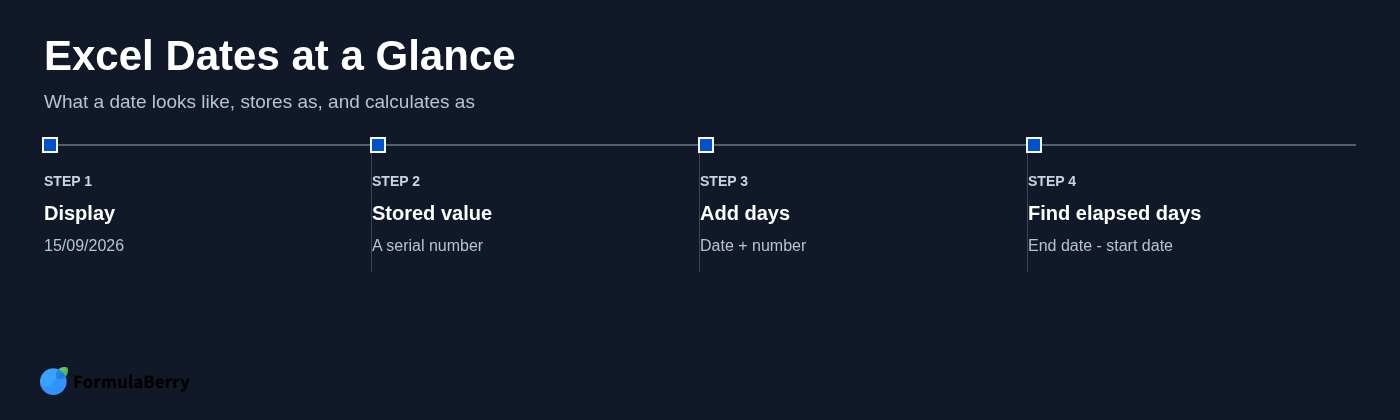
Excel does not store most dates as words such as "15 September 2026." It stores them as serial numbers. A date is a whole number representing a day, while a time is stored as a fraction of a day.

That is why date arithmetic works so naturally. If cell A2 contains a real Excel date, =A2+10 adds ten calendar days. If B2 contains a later date, =B2-A2 returns the number of days between them. The date may display as 15/09/2026, but behind the scenes Excel is working with a number.

Most Windows versions of Excel use the 1900 date system, which counts dates from an early baseline. You do not need to memorize that baseline to use date formulas well. The useful point is that a genuine date is numeric, so Excel can sort it, subtract it, filter it, and use it in calculations.

A date-looking value is not always a real date. For example, an imported value such as 15/09/2026 may be text rather than a date serial number. It can look correct on screen but fail when you try to subtract it from another date or sort a column chronologically.

Regional settings create another common problem. In one locale, 03/04/2026 may mean 3 April. In another, it may mean March 4. Formatting is separate from storage, but Excel's interpretation of typed or imported text can depend on your locale. When accuracy matters, build dates with DATE or use an unambiguous source format.

Quick start: the five date formulas most people need

Formula	What it returns	Practical use
=TODAY()	The current date	Today's tasks, overdue flags, daily reports
=DATE(2026,9,15)	A reliable date value for 15 September 2026	Creating dates without locale ambiguity
=A2+10	The date ten calendar days after A2	Simple deadlines and follow-up dates
=B2-A2	The number of elapsed calendar days	Measuring time between two dates
=EDATE(A2,1)	The date one calendar month after A2	Monthly renewals, billing, and reporting cycles

These formulas cover a surprising amount of everyday spreadsheet work. The sections below explain when each is appropriate and where simple-looking date logic can go wrong.

Create dates reliably with DATE, TODAY, NOW, and DATEVALUE

There are several ways to place dates in an Excel workbook, but they are not interchangeable. The best method depends on whether the date is fixed, changes automatically, comes from separate input fields, or arrives as imported text.

Build a date from year, month, and day cells with DATE

DATE is the safest formula for constructing a date because it tells Excel exactly which number is the year, month, and day. If A2 contains a year, B2 contains a month number, and C2 contains a day number, use:

=DATE(A2,B2,C2)

For a fixed date, the same approach looks like this:

=DATE(2026,9,15)

This is much safer than assembling text such as A2&"/"&B2&"/"&C2, which can be interpreted differently depending on local settings. It is especially useful in forms, imports, budget templates, and reports where year, month, and day are stored in separate columns.

DATE also normalizes overflow values. For example, a month input of 13 rolls into the next year, and a day value beyond the end of a month rolls into the next month. That behavior can be helpful in controlled calculations, but it can also hide bad input. If users enter source data manually, validate month and day values rather than relying on DATE to correct them silently.

Insert the current date automatically with TODAY and NOW

Use =TODAY() when you need the current date without a time. It updates whenever the workbook recalculates, making it useful for task trackers, aging reports, and formulas that identify overdue work.

Use =NOW() when you need both the current date and current time. Because it includes time, it can produce unexpected results if you subtract it from a date-only value. Format the cell as a date and time when that detail matters.

Neither formula creates a permanent timestamp. If you enter =TODAY() on Monday, it will show Tuesday after recalculation on Tuesday. For a static entry, use a keyboard shortcut instead: Ctrl+; inserts the current date, and Ctrl+Shift+; inserts the current time in Excel for Windows.

A common mistake is using TODAY for an "order received" date that must never change. Use a static timestamp for historical records; use TODAY only when the calculation should stay tied to the actual current day.

Convert imported date text with DATEVALUE

DATEVALUE converts recognizable text into a real Excel date serial number. For example:

=DATEVALUE("15/09/2026")

Once converted, the result may display as a number until you apply a date format. That does not mean the formula failed. It means Excel has stored a valid date but is displaying the underlying serial value.

DATEVALUE is sensitive to locale. A text string that works on a system expecting day/month/year may fail or be misread on a system expecting month/day/year. Use it only when the source text is already unambiguous for your Excel settings.

For unreliable imports, split the text into year, month, and day components and reconstruct the date with DATE. If the source system can export dates in a consistent ISO-like pattern such as 2026-09-15, that is usually easier to manage than ambiguous slash-separated dates.

Format dates as dd/mm/yyyy without changing the underlying value

Changing a date format changes how a date looks, not what it is. A cell can display 15/09/2026, 15 Sep 2026, or Tuesday, 15 September 2026 while retaining exactly the same serial number underneath.

To format a date as dd/mm/yyyy, select the cells, open Format Cells, choose Custom, and enter:

dd/mm/yyyy

This is the right answer when you need Excel to show a date in day-month-year order while preserving its ability to calculate.

Use custom number formats for local and reporting-friendly dates

Custom number formats let you make date columns easier to read without changing the underlying value. Useful options include:

• dd/mm/yyyy - 15/09/2026
• d mmm yyyy - 15 Sep 2026
• dd-mmm-yyyy - 15-Sep-2026
• mmm-yy - Sep-26
• dddd, d mmmm yyyy - Tuesday, 15 September 2026

For reports shared across regions, dd-mmm-yyyy is often clearer than 15/09/2026 because the month is written as text. It removes most day/month ambiguity without making the date column excessively wide.

Do not convert a valid date to text just to control how it looks. Formatting is the cleaner solution because filters, sorting, date subtraction, and formulas such as EDATE will continue to work.

Use TEXT only when the result should be text

The TEXT function converts a value into text with a chosen display pattern:

=TEXT(A2,"dd/mm/yyyy")

This is useful when creating a label, file name, export field, or message such as:

="Report due: "&TEXT(A2,"dd-mmm-yyyy")

However, TEXT does not return a date. It returns characters that look like a date. That makes it the wrong choice for a date column that will later be sorted, compared, or used in arithmetic. Keep the original value as a real date and use formatting whenever calculations are still needed.

Add or subtract days from a date

Adding calendar days is the simplest type of Excel date calculation. Because dates are serial numbers, the formula is ordinary addition. But it counts every calendar day, including weekends and holidays. That distinction matters for delivery dates, service-level agreements, and project plans.

Add a fixed number of calendar days

If A2 contains a date, add ten days with:

=A2+10

To add a variable number of days stored in B2, use:

=A2+B2

To move backward, subtract instead:

=A2-10

If the result appears as a number such as 46280, the formula is probably correct. Apply a date format to the result cell. As covered earlier, Excel is showing the serial number rather than the formatted date.

Auto-populate dates based on another cell

For a recurring sequence or due-date column, reference the source date and add the required interval. If an order date is in A2 and the standard turnaround is seven calendar days, use:

=IF(A2="","",A2+7)

The IF check is important. Without it, blank rows can display misleading dates based on Excel's zero-date behavior. In a more flexible tracker, use a turnaround-days column:

=IF(OR(A2="",B2=""),"",A2+B2)

Here, A2 is the order date and B2 is the required number of days. The formula stays blank until both inputs exist, then calculates the due date automatically.

Use this pattern for invoice follow-ups, return deadlines, event preparation, and customer commitments. If the agreement is defined in business days rather than calendar days, skip simple addition and use WORKDAY instead.

FormulaBerry

For straightforward formulas, typing =A2+10 is faster than asking for help. The value of FormulaBerry is in turning a plain-language requirement into the correct formula when the rule has conditions, blank handling, date offsets, or spreadsheet-specific references.

For example, you can describe a requirement such as: "If the order date is blank, leave the result blank; otherwise add the number of days in B2." The assistant can generate a formula such as =IF(OR(A2="",B2=""),"",A2+B2), explain what it does, or help correct a version that is returning an error. For more involved formula work, see the Excel Formula Generator: Create, Explain, and Fix Formulas.

It is a formula assistant, not a replacement for Excel or Google Sheets. Choose it when you need help expressing a date rule as a formula, particularly if you do not want to troubleshoot nested IF statements, date functions, or cell references from scratch.

Add months and years without breaking month-end dates

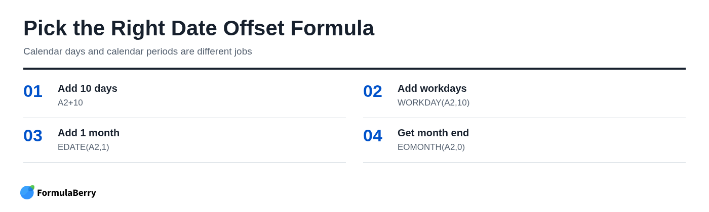
Adding 30 days is not the same as adding one month. A 30-day offset from January 31 lands in early March in many years, while a one-month billing cycle should usually land at the end of February.

Use calendar-aware functions when the rule is monthly, quarterly, annual, or tied to the end of a reporting period.

Move by whole months with EDATE

EDATE shifts a date by a specified number of whole months:

=EDATE(A2,1)

This returns the date one month after A2. To move back three months, use:

=EDATE(A2,-3)

EDATE handles short months sensibly. If A2 is January 31, adding one month returns the final valid day of February: February 28 in a non-leap year or February 29 in a leap year. This makes it a strong choice for subscriptions, payment schedules, monthly reviews, and renewal dates.

Find month ends with EOMONTH

EOMONTH returns the last day of a month. To find the end of the month containing the date in A2, use:

=EOMONTH(A2,0)

To find the end of the following month, use:

=EOMONTH(A2,1)

For example, a finance team can use EOMONTH to assign every transaction to its reporting cutoff. A project manager can use it to create a recurring "submit by month end" deadline without manually checking whether a month has 28, 29, 30, or 31 days.

Add years with DATE while controlling leap-day behavior

To move a date forward one year, you can rebuild it with:

=DATE(YEAR(A2)+1,MONTH(A2),DAY(A2))

This approach makes the logic clear, but check February 29 source dates. If A2 is February 29 and the next year is not a leap year, DATE normalizes the invalid day into March. That may not match your business rule.

For many annual schedules, this is shorter:

=EDATE(A2,12)

EDATE is often preferable because its month-end behavior is practical for recurring calendar periods. Still, decide explicitly what should happen to leap-day anniversaries: February 28, March 1, or another policy-based date.

Calculate date differences in days, months, and years

Date difference formulas answer different questions. "How many days have passed?" is not the same as "How many complete months have passed?" Choose the formula based on the rule you are measuring.

Find the number of days between two dates

For calendar-day elapsed time, subtract the start date from the end date:

=B2-A2

If A2 is the start date and B2 is the end date, the result is the number of days between them. If B2 comes before A2, the answer is negative. That can be useful for detecting invalid date order, but you can wrap the calculation in ABS if you only need the magnitude:

=ABS(B2-A2)

Simple subtraction normally excludes the start date. If a business rule counts both the start and end date, add one:

=B2-A2+1

Do not add one by habit. For example, an event that starts on Monday and ends on Tuesday spans one elapsed day, but it covers two calendar dates. The correct approach depends on the rule.

Use DATEDIF for completed months and years

DATEDIF calculates completed units between two dates. Common versions are:

• =DATEDIF(A2,B2,"d") - completed days
• =DATEDIF(A2,B2,"m") - completed months
• =DATEDIF(A2,B2,"y") - completed years

DATEDIF is useful for age, tenure, subscription duration, and contract periods because it distinguishes complete months or years from partial ones. A period from January 15 to February 14 is not a complete month; from January 15 to February 15, it is.

The start date must be earlier than or equal to the end date. If the dates are reversed, DATEDIF returns an error rather than a negative count. Validate chronology first if users can enter both dates manually.

Use YEARFRAC when a partial year matters

For prorating, accrued service, or calculations where a partial year should count, use:

=YEARFRAC(A2,B2)

The result is a decimal. For example, 0.5 represents roughly half a year, depending on the date range and calculation basis.

YEARFRAC accepts an optional basis argument that controls how days are counted. That detail matters in finance, where actual/actual, actual/365, and 30/360 conventions can produce different answers. Match the basis to the contract, accounting policy, or business rule rather than choosing one arbitrarily.

Calculate working days, weekends, and holidays

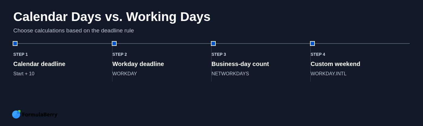
Many real deadlines are not calendar deadlines. "Respond within ten days" may mean ten calendar days. "Resolve within ten business days" means weekends and specific holidays should be excluded. A simple +10 formula cannot make that distinction.

Count business days with NETWORKDAYS

Use NETWORKDAYS to count working days between two dates:

=NETWORKDAYS(A2,B2,$H$2:$H$20)

A2 is the start date, B2 is the end date, and H2:H20 contains holiday dates to exclude. The formula assumes Saturday and Sunday are weekends and includes both endpoints when they are workdays.

Maintain holidays in a dedicated range rather than typing holiday dates directly into every formula. Keep the entries as real Excel dates, not text. That makes the list reusable across trackers, reports, and departments.

Set a due date with WORKDAY and WORKDAY.INTL

Use WORKDAY to calculate a future or past workday date:

=WORKDAY(A2,10,$H$2:$H$20)

This returns the date ten working days after the start date in A2, excluding Saturdays, Sundays, and the holiday range.

If your workweek is not Saturday-Sunday, use WORKDAY.INTL. For example:

=WORKDAY.INTL(A2,10,7,$H$2:$H$20)

In this example, the weekend code 7 represents Friday and Saturday as weekend days. WORKDAY.INTL also supports custom weekend patterns for schedules that do not follow a standard regional workweek.

The most important step is not choosing the function. It is confirming the deadline rule with the people who use the sheet. As we covered in the previous sections, calendar days, whole months, and workdays produce different results even when the phrase "due in ten days" sounds straightforward.

Extract date parts and build date-based logic

Once dates are stored correctly, Excel can turn them into useful components for reporting, filtering, scheduling, and status rules. These functions preserve the connection to the original date while giving you the part you need.

Return the day, month, year, weekday, and week number

Use these formulas to extract numeric date components:

• =DAY(A2) - day of the month
• =MONTH(A2) - month number from 1 to 12
• =YEAR(A2) - four-digit year
• =WEEKDAY(A2) - day-of-week number
• =WEEKNUM(A2) - week number in the year

WEEKDAY needs particular care because the numbering can vary. By default, Sunday is 1 and Saturday is 7. If you want Monday as 1 and Sunday as 7, use:

=WEEKDAY(A2,2)

That return type is often easier for weekday-based formulas. For example, values 1 through 5 represent Monday through Friday, which is convenient for standard business-day logic.

Create readable month and weekday labels

For display labels, TEXT is useful:

=TEXT(A2,"mmmm")

returns a full month name, while:

=TEXT(A2,"dddd")

returns a full weekday name.

These labels work well in dashboards and report headers. But remember that they are text. For calculations, filtering logic, or reliable chronological grouping, MONTH, YEAR, and WEEKDAY are usually better because they return numeric values. For counting records that match date-related criteria, you can also use the COUNTIF formula in Google Sheets with date ranges or extracted values.

Flag overdue, upcoming, and current-period dates

A simple overdue flag can compare a due date against TODAY:

=IF(A2="","",IF(A2<TODAY(),"Overdue","Open"))

The blank check prevents empty rows from being marked overdue. To identify work due in the next seven days, use AND:

=IF(A2="","",IF(AND(A2>=TODAY(),A2<=TODAY()+7),"Due in 7 days",""))

You can combine these rules into a broader status formula, but keep the priority clear. An overdue item should be checked before an upcoming one. A date due today usually deserves its own label rather than being grouped with work due later in the week.

Worked example: build a deadline tracker that handles blanks, holidays, and status

A formula list is useful, but the real value comes from combining date logic into a spreadsheet people can use every day. This example builds a project deadline tracker that calculates holiday-aware due dates and gives each task a clear status.

Set up the input columns and holiday list

Create a task table with these columns:

• Task
• Start Date
• SLA Workdays
• Due Date
• Days Remaining
• Status

Place your holiday list in H2:H20, or another dedicated range. Include only real date values in that range. A typed label such as "Christmas Day" is not enough for WORKDAY or NETWORKDAYS; Excel needs the date itself.

Suppose a task starts on 15 September 2026 and has an SLA of 10 working days. The due date should skip weekends and any dates listed in the holiday range.

Write the due-date formula without false dates on blank rows

In the Due Date column of an Excel table, use:

=IF(OR([@[Start Date]]="",[@[SLA Workdays]]=""),"",WORKDAY([@[Start Date]],[@[SLA Workdays]],$H$2:$H$20))

The formula works in a deliberate sequence. First, it checks whether Start Date or SLA Workdays is blank. If either value is missing, it returns an empty result rather than inventing a date. If both inputs exist, WORKDAY adds the required number of working days and excludes the holiday range.

If Friday and Saturday are nonworking days for your team, replace WORKDAY with WORKDAY.INTL and add the appropriate weekend code:

=IF(OR([@[Start Date]]="",[@[SLA Workdays]]=""),"",WORKDAY.INTL([@[Start Date]],[@[SLA Workdays]],7,$H$2:$H$20))

This is the kind of formula where a small wording change can matter. "Ten business days after the start date" may differ from "the tenth day including the start date." Test the formula with a known date and confirm the policy before filling it down an operational tracker.

Calculate days remaining and a useful status label

If the business wants to see calendar days remaining until the due date, use:

=IF([@[Due Date]]="","",[@[Due Date]]-TODAY())

For a working-day countdown instead, use:

=IF([@[Due Date]]="","",NETWORKDAYS(TODAY(),[@[Due Date]],$H$2:$H$20)-1)

The minus one avoids counting today as a remaining day when today is a workday. Whether that is correct depends on your reporting convention, so document the rule in the tracker.

A practical status formula based on calendar days remaining is:

=IF([@[Due Date]]="","",IF([@[Due Date]]<TODAY(),"Overdue",IF([@[Due Date]]=TODAY(),"Due today",IF([@[Due Date]]<=TODAY()+7,"Due soon","On track"))))

This formula checks blank values first, then overdue work, then items due today, then work due within seven days. The order matters. If you test "due within seven days" before "overdue," an overdue task may be assigned the wrong label.

Fix common Excel date formula errors

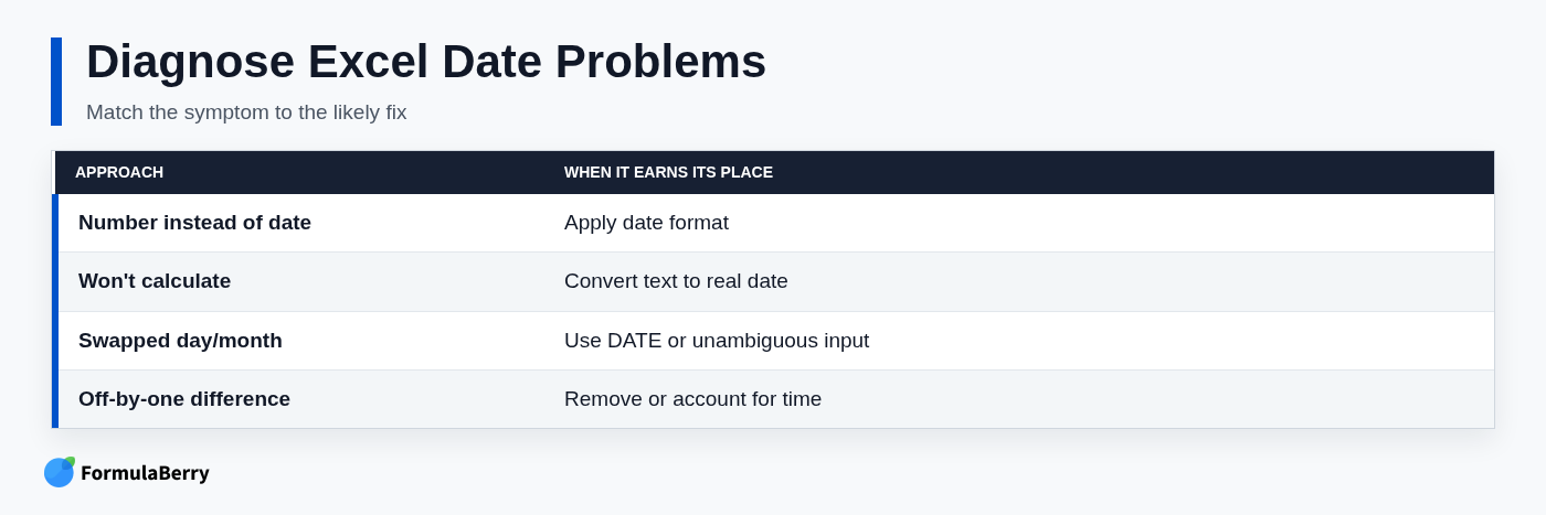
When date formulas misbehave, start by checking the value type before rewriting the formula. The usual causes are text dates, regional ambiguity, incorrect formatting, hidden times, or an invalid date order.

A date displays as a number

If a cell displays something like 46280 after a date formula, Excel has probably returned a valid serial number. The issue is formatting, not calculation.

Select the cell and apply a date number format, such as dd/mm/yyyy or dd-mmm-yyyy. Do not wrap the formula in TEXT unless you explicitly need a text result.

Dates will not sort, subtract, or calculate

Dates that refuse to sort properly or return errors in subtraction are often stored as text. One quick test is:

=ISNUMBER(A2)

TRUE suggests Excel recognizes the cell as a numeric date or date-time. FALSE suggests text or another nonnumeric value. Alignment can offer a clue too, since text often aligns left by default, but do not rely on alignment alone because cell formatting can override it.

For consistent, unambiguous imported date text, DATEVALUE may be enough. For a consistently structured import, Excel's Text to Columns tool can convert a full column. For mixed or ambiguous formats, reconstruct the values with DATE from separate year, month, and day components. That is slower to set up, but more reliable than guessing.

Day and month are swapped or the formula returns #VALUE!

Values such as 03/04/2026 are risky because both interpretations are valid dates. Excel may read the first number as the month or day based on regional settings. A value like 15/09/2026 may return #VALUE! in a month/day locale because Excel cannot interpret 15 as a month.

Where possible, use an unambiguous source pattern such as 2026-09-15. When building dates in formulas, use =DATE(year,month,day) rather than parsing an ambiguous text string. DATE makes your intent explicit and avoids locale-dependent interpretation.

Time stamps make date differences seem off by one

Date-times include a fractional portion. For example, 15 September 2026 at noon is stored as the date serial number plus 0.5. Two cells can display the same date format while holding different hidden times.

Suppose A2 is 15/09/2026 at 23:00 and B2 is 16/09/2026 at 01:00. They are on different displayed dates, but only two hours apart. Conversely, subtracting date-times can return 0.08 instead of the whole-day result you expected.

If the business rule ignores time, remove it with INT:

=INT(A2)

For a date-only difference, use:

=INT(B2)-INT(A2)

Do not strip times automatically if the time is operationally meaningful. The correct formula should reflect whether you are measuring calendar dates, full 24-hour periods, or working hours.

A practical formula cheat sheet for everyday Excel date tasks

Copy-ready formulas and when to use them

Task	Formula	Replace as needed
Show today's date	=TODAY()	No arguments needed
Create a date from components	=DATE(A2,B2,C2)	A2 year, B2 month, C2 day
Add calendar days	=A2+10	10 with your day count
Add variable calendar days	=A2+B2	A2 date, B2 day count
Subtract calendar days	=A2-10	10 with your day count
Add one month	=EDATE(A2,1)	1 with months to add or subtract
Find current month end	=EOMONTH(A2,0)	0 with the month offset
Find elapsed days	=B2-A2	A2 start, B2 end
Find complete months	=DATEDIF(A2,B2,"m")	A2 start, B2 end
Set a workday due date	=WORKDAY(A2,10,$H$2:$H$20)	10 and the holiday range
Count business days	=NETWORKDAYS(A2,B2,$H$2:$H$20)	Start, end, and holiday range
Return the month number	=MONTH(A2)	A2 with your date cell
Return Monday-based weekday number	=WEEKDAY(A2,2)	A2 with your date cell
Display as dd/mm/yyyy	dd/mm/yyyy	Apply as a custom number format
Create a text date label	=TEXT(A2,"dd/mm/yyyy")	A2 with your date cell

Use the right date formula for the deadline you actually mean

The best Excel date formula depends on the rule behind the date. Use +10 for ten calendar days, WORKDAY for ten working days, EDATE for one calendar month, and DATEDIF when you need completed months or years.

Store dates as real Excel values, keep display formatting separate from calculation logic, and test formulas against awkward cases such as month end, February 29, weekends, blank rows, and holidays. Those edge cases reveal whether a formula reflects the actual business rule or merely looks right in a normal month.

If you can describe the spreadsheet task in plain language, FormulaBerry can help generate, explain, or correct the Excel or Google Sheets formula that matches it.