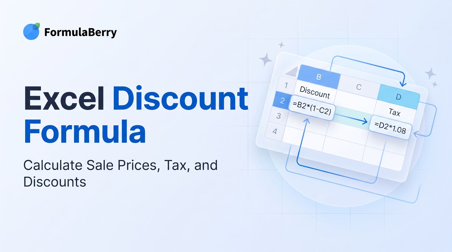
A discount formula looks simple until a spreadsheet returns a negative price, taxes the wrong amount, or shows 0.2 when you expected 20%. The fix is usually not advanced Excel knowledge. It is using the right percentage value and calculation order.

This guide shows how to calculate discount amounts, sale prices, discount percentages, and tax-adjusted final prices in Excel. The examples work the same way in Google Sheets.

Calculate the discounted sale price with one Excel formula

The standard Excel discount formula for a sale price is:

=A2*(1-B2)

In this example, A2 contains the original price and B2 contains the discount rate. If the original price is $100 and the discount is 20%, the formula returns $80.

You can also write a fixed discount directly in the formula:

=A2*(1-20%)

Both approaches work. Keeping the discount in a cell is usually better for a worksheet with many products because you can update rates without editing every formula.

For a quick Excel discount formula example, enter 100 in A2 and 20% in B2. Then enter =A2*(1-B2) in C2. Excel calculates an $80 sale price.

Set up your price and discount columns correctly

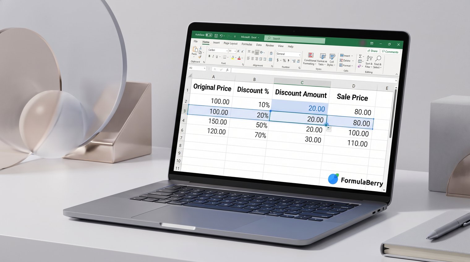
A clear worksheet prevents most discount-calculation mistakes. Use one row per product and keep the price, discount, tax, and results in separate columns.

Product	List Price	Discount %	Discount Amount	Sale Price	Tax Rate	Final Price
Office Chair	$250.00	30%	$75.00	$175.00	8%	$189.00

For the first data row, your formulas might be:

• Discount Amount: =B2*C2
• Sale Price: =B2*(1-C2)
• Final Price, after tax: =E2*(1+F2)

Format list price, discount amount, sale price, and final price as Currency. Format the discount and tax columns as Percentage. For more ways to format numeric results and dates, see this Excel TEXT formula guide. Clear formatting makes the sheet easier to audit and helps you spot incorrect entries quickly.

These formulas use relative cell references, meaning Excel changes the row number as you copy them downward. A formula entered as =B2*C2 in row 2 becomes =B3*C3 in row 3.

Enter discount rates as percentages, not whole numbers

Enter a 20% discount as 20% or 0.2, not as 20. In Excel, 20% and 0.2 represent the same underlying value. Percentage formatting displays 0.2 as 20% without changing the calculation.

Typing 20 into a standard sale-price formula such as =A2*(1-B2) tells Excel to subtract 20 times the original price. That creates an invalid negative result for most ordinary prices.

A good default is to type 20% directly into the cell. It is readable at a glance and much harder for someone reviewing the sheet to misunderstand.

Calculate the discount amount separately

The discount amount is the money the customer saves. Calculate it with:

=A2*B2

If A2 contains $250 and B2 contains 30%, the result is $75. The sale price is not $75; it is the original $250 minus the $75 discount, or $175.

Keeping these values separate is useful for invoices, quotes, approval workflows, and reports where you need to show both the markdown and the post-discount price.

Find 20%, 30%, or any percentage of a number

To calculate 30% of 250, use:

=250*30%

Excel returns 75. In a worksheet, the more flexible version is =A2*B2, where A2 holds the number and B2 holds the percentage. For additional examples, see this Excel percentage formula guide.

The same pattern applies to a 20% discount formula in Excel: multiply the price by 20% to find the amount discounted, or multiply the price by (1-20%) to find the remaining sale price.

Copy the discount formula down multiple rows

Enter your formulas in the first product row, then copy them down for the rest of the list. For example, if column B is List Price and column C is Discount %, enter these formulas in row 2:

• Discount Amount in D2: =B2*C2
• Sale Price in E2: =B2*(1-C2)

Select D2 or E2, then use the small square at the lower-right corner of the selected cell, called the fill handle. Drag it down through the needed rows. If an adjacent column has continuous data, double-clicking the fill handle usually fills the formula down automatically.

Excel adjusts relative references for each row. For example, =B2*(1-C2) becomes =B3*(1-C3) on the next line. Do not manually rewrite the formula for every product unless each row follows a genuinely different pricing rule.

Calculate the discount percentage from original and sale prices

Sometimes you know the list price and sale price but need to find the markdown percentage. Use this formula:

=(A2-B2)/A2

Here, A2 is the original price and B2 is the sale price. For a product reduced from $100 to $80, the formula returns 0.2. Format the result cell as Percentage to display 20%.

The original price must be the base value because the question is, "What percentage of the original price was removed?" This is different from other percentage-change calculations that may use a different starting or comparison value.

Avoid reversing the subtraction order

Use original price minus sale price, not sale price minus original price. The reversed formula produces a negative percentage:

=(B2-A2)/A2

A quick accuracy check is simple: if the sale price is lower than the original price, the discount percentage should be positive.

Add sales tax after applying a discount

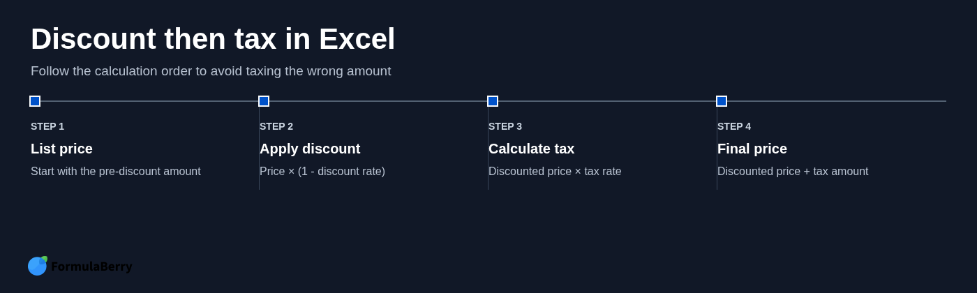
In most pricing scenarios, calculate the discount first and apply sales tax to the discounted price. The combined formula is:

=A2*(1-B2)*(1-C2)

In this formula, A2 is the list price, B2 is the discount rate, and C2 is the tax rate. For example, a $100 item with a 20% discount and 8% sales tax becomes $86.40:

• $100 x (1 - 20%) = $80 sale price
• $80 x (1 + 8%) = $86.40 final price

Tax rules can vary by jurisdiction, product type, and store policy. Follow the applicable rule for your transaction, especially when preparing invoices or customer-facing quotes.

Calculate the tax amount and final price in separate cells

A one-cell formula is convenient, but separate columns are easier to verify. If D2 contains the discounted sale price and C2 contains the tax rate, use:

• Sale Price in D2: =A2*(1-B2)
• Tax Amount in E2: =D2*C2
• Final Price in F2: =D2+E2

This approach is more audit-friendly because you can see exactly how much discount and tax were applied. It is usually the better choice for receipts, invoices, budget approvals, and shared pricing files.

Use one formula for a final price with discount and tax

For a simple price list, use this compact final-price formula:

=A2*(1-B2)*(1-C2)

With a $100 list price, a 20% discount, and 8% tax, Excel calculates $86.40. This is efficient when you only need the customer total.

Use separate discount, sale-price, and tax columns when someone needs to review the calculation or when prices are used in invoices and reports. A shorter formula is not always a better worksheet. Transparency matters when another person must confirm the numbers.

Apply different discount rules with IF or IFS

Fixed discounts are easy. Tiered discounts need a condition. For example, to apply 10% off only when the list price is at least $100, use:

=IF(A2>=100,A2*(1-10%),A2)

If A2 is $100 or more, Excel calculates a 10% discount. If it is less than $100, Excel returns the full original price.

For multiple tiers, an IFS formula can work well for a small set of rules:

=IFS(A2>=500,A2*(1-20%),A2>=250,A2*(1-15%),A2>=100,A2*(1-10%),TRUE,A2)

This applies 20% off at $500 or more, 15% off at $250 or more, 10% off at $100 or more, and no discount below $100. Put the highest threshold first so a $600 item receives 20%, not 10%.

Once discount rules expand beyond a few tiers, store thresholds and rates in a separate table rather than embedding every percentage in a long formula.

Keep the discount rate separate when possible

The safest design is to calculate or retrieve the applicable rate in one cell, then reuse the standard sale-price formula:

=B2*(1-C2)

That keeps pricing logic visible. It also prevents a common maintenance problem: changing a policy from 10% to 12% but missing one hard-coded 10% inside a formula elsewhere in the workbook.

Handle common discount formula errors

Most Excel discount formula problems come from a few predictable mistakes:

• Entering 20 instead of 20%: Use 20% or 0.2 as the discount rate. A whole-number 20 is not a 20% discount.
• Subtracting a percentage directly from a price: =100-20% returns 99.8, not $80. Multiply the price by the percentage or by the remaining percentage instead.
• Calculating tax from the list price: If tax applies after the discount, calculate tax from the sale price, not the original price.
• Using the wrong cell format: A value of 0.2 is correct for a percentage but needs Percentage formatting to display as 20%.
• Getting an unexpected date or currency display: Change the cell format to General, Number, Percentage, or Currency as appropriate.

If one tax rate or discount rate applies to every row, use an absolute reference so it does not move when copied. For example, if the tax rate is stored in B1, use:

=A2*(1-$B$1)

The dollar signs lock B1 in place. Without them, copying the formula down changes the reference to B2, B3, and so on.

Build a reusable discount calculator sheet

A reusable calculator gives you more than a one-off percentage answer. It creates a pricing workflow you can check, update, and share without rebuilding formulas each time.

Include these columns:

• Product
• Original Price
• Discount %
• Discount Amount
• Sale Price
• Tax %
• Tax Amount
• Final Price

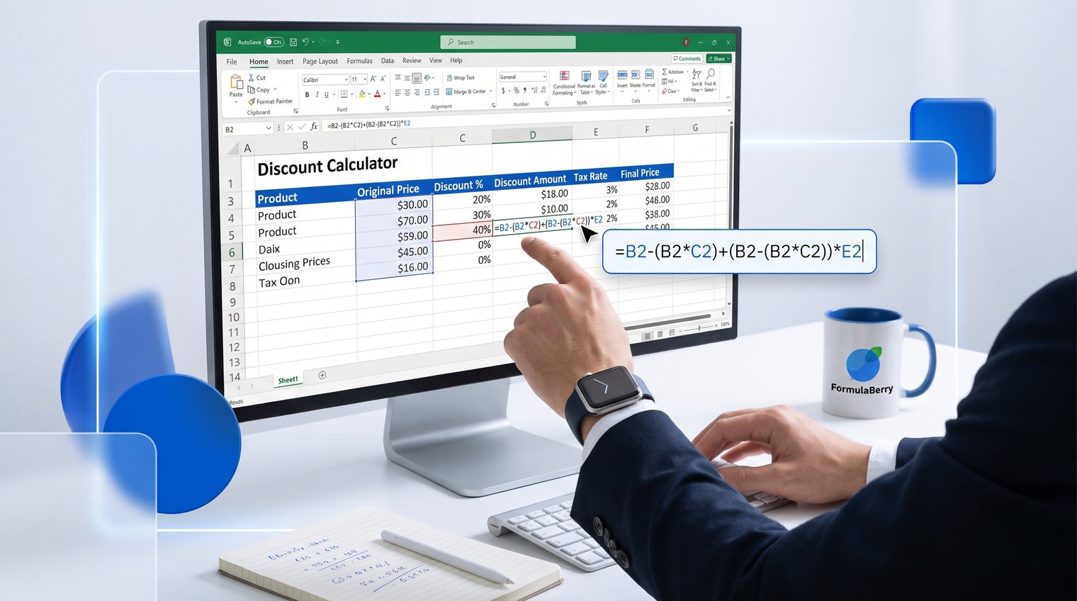
Use =B2*C2 for Discount Amount, =B2*(1-C2) for Sale Price, =E2*F2 for Tax Amount, and =E2+G2 for Final Price. Format price fields as Currency and rate fields as Percentage.

For ongoing work, convert the range into an Excel Table. Select any cell in the range, then use Insert > Table and confirm that your headers are included. Excel will extend formulas and formatting automatically when you add new products.

Apply the formula that matches your pricing task

Use the formula that answers the number you actually need:

• Discount amount: price x discount rate, or =A2*B2
• Sale price: price x (1 - discount rate), or =A2*(1-B2)
• Final price with tax: price x (1 - discount rate) x (1 + tax rate), or =A2*(1-B2)*(1+C2)

Before trusting the result, check that discount and tax cells are formatted as percentages and that tax is being calculated from the correct price. Those two checks catch the majority of spreadsheet pricing errors.

If you need to turn a specific pricing policy into an Excel or Google Sheets formula, FormulaBerry can generate, explain, or help correct the formula from a plain-language request.