
A spreadsheet can look finished while hiding a formula mistake that changes every total, forecast, or commission payment underneath it. The fastest way to work with Excel formulas is not memorizing hundreds of functions. It is knowing how to get the right kind of help at the right moment: while creating a formula, decoding an existing one, or finding the exact point where a result went wrong.
This guide covers practical Excel formula assistance from the basics through debugging complex logic. You will learn how to use Excel's built-in features, how to ask for formula help clearly, and how to validate every result before it affects a real report.
What Excel Formula Assistance Means - and When to Use It
Excel formula assistance is the combination of tools and methods that help you create, understand, and repair formulas. That includes Excel's autocomplete and function dialogs, formula auditing tools such as Evaluate Formula, and AI tools that translate a plain-English request into a formula.
Assistance speeds up the mechanical part of formula work, but it cannot verify whether your source data is accurate or whether the business rule itself is correct. A formula can be syntactically perfect and still calculate the wrong thing because it references the wrong column, uses the wrong date rule, or treats blanks differently than your process requires.
Quick start: choose the right kind of help
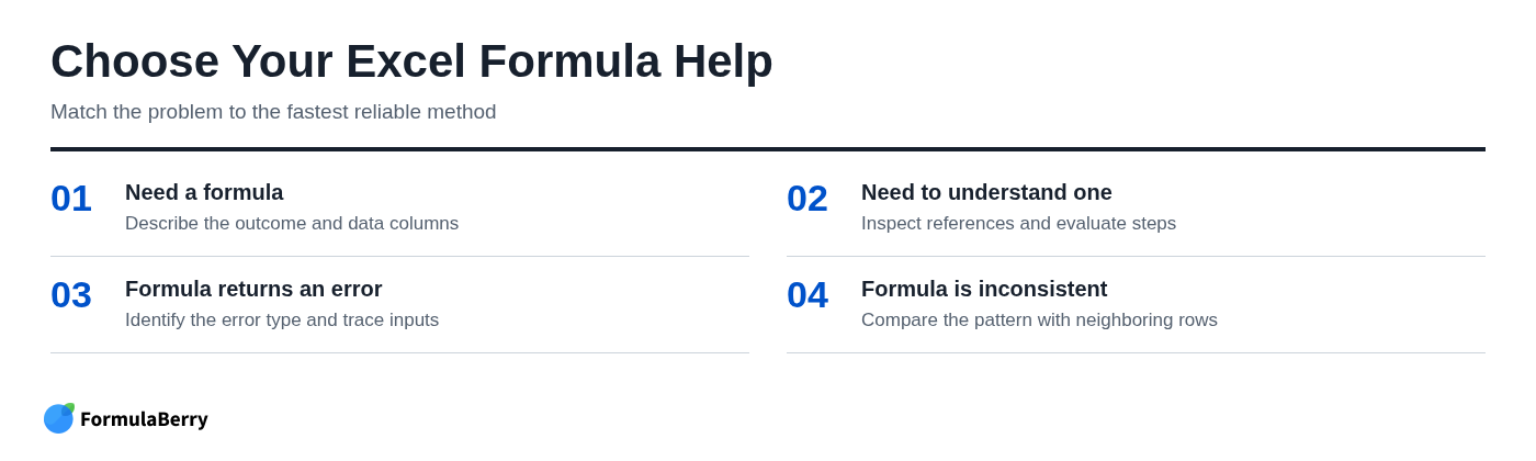
Start by identifying the actual problem. If you know the function but keep getting the syntax wrong, Excel's autocomplete, tooltips, and Insert Function dialog are usually enough. If a formula already exists but returns an error or a suspicious number, use auditing tools to inspect its inputs and calculation steps.
If the difficulty is turning a business request into formula logic, natural-language formula assistance is often the better starting point. Describe the outcome, the relevant columns, the conditions, and how blanks or missing matches should behave. Then test the suggested formula with known examples before filling it down. For more help with this workflow, see the Excel Formula Generator: Create, Explain, and Fix Formulas.
- Create: Define the desired output, source columns, and conditions.
- Understand: Identify the outer function and work inward through each nested section.
- Fix: Start with the error type or unexpected result, then trace references and test inputs.
Formula Fundamentals You Need Before Asking for Help
You do not need an exhaustive Excel formulas list to work confidently. But you do need enough vocabulary to recognize what a formula is doing and to describe what you need when asking for help.
Every formula begins with an equals sign. It can contain functions such as SUM or IF, arguments inside parentheses, operators such as +, -, *, and /, fixed values called constants, and references to cells or ranges. In =SUM(B2:B10), SUM is the function and B2:B10 is the range argument.
Relative, absolute, and mixed references
Cell references determine what moves when you copy a formula. This is one of the most important concepts behind filling formulas across an entire column.
- A1 is a relative reference. It changes when copied. Copy =B2*C2 down one row, and Excel changes it to =B3*C3.
- $A$1 is an absolute reference. Both the column and row stay locked wherever you copy the formula.
- A$1 locks row 1 but allows the column to change.
- $A1 locks column A but allows the row to change.
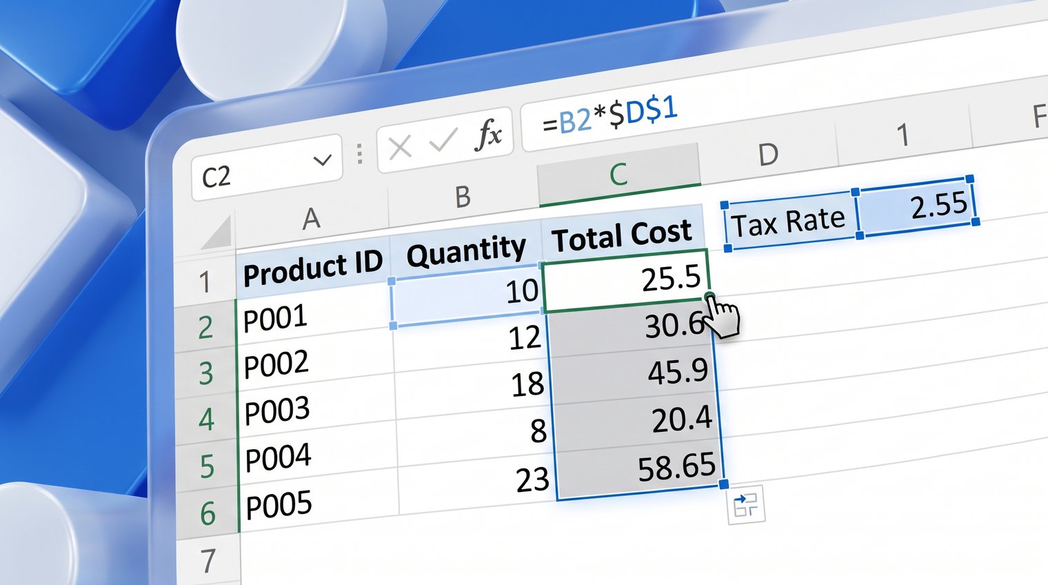
Imagine a sales sheet where column B contains revenue and cell F1 contains a commission rate of 8%. The formula in C2 might be =B2*$F$1. Revenue should move from B2 to B3 to B4 as you copy down, but the rate must continue pointing to F1. Forgetting the dollar signs is a common reason a formula works in the first row and quietly fails below it.
How Excel reads a formula
Excel follows an order of operations. It resolves parentheses first, then performs multiplication and division before addition and subtraction. A formula such as =A2+B2*C2 is not the same as =(A2+B2)*C2, so use parentheses whenever the intended grouping could be unclear.
Ranges also matter. =SUM(B2:B10) includes every cell from B2 through B10, while =SUM(B2,B10) adds only two cells. Excel distinguishes numbers, text, dates, blanks, and errors, and those data types affect results. A date that looks correct but is stored as text, for example, may not work in a date calculation.
This is why a valid formula can still return the wrong business result. Excel only follows the instructions it receives; it does not know that a text value was intended to be a number or that a lookup should use the current month rather than the prior month.
Create Formulas in Excel with Built-In Assistance
Excel provides useful guidance while you enter formulas. These features reduce spelling and syntax errors, especially when you are working with unfamiliar functions. Exact menu labels and available functions can vary by your Excel version and platform, but the underlying workflow is similar.
Formula autocomplete and function tooltips
Type an equals sign followed by the first letters of a function, such as =SU, and Excel can suggest matching functions. Select one from the list and Excel inserts the function name and opening parenthesis for you.
As you enter arguments, Excel displays a tooltip showing the function's expected order. For example, XLOOKUP expects a lookup value, a lookup array, and a return array before optional arguments. This is particularly helpful with nested formulas, where one missing comma or closing parenthesis can make the whole formula fail.
Tooltips explain syntax, not intent. Excel can tell you where an argument belongs, but it cannot tell you whether you should use an exact match, whether a missing result should remain blank, or whether the lookup table is the correct source of truth.
Insert Function and Formula Builder
The Insert Function dialog is useful when you know the outcome you want but not the function name. Search with a description such as "count cells that meet a condition" or browse a category such as Math & Trig, Logical, Lookup & Reference, or Date & Time.
It also provides an argument-by-argument view, which can be easier to use than typing a long formula directly into the formula bar. Before accepting a result, read the function description and confirm what each argument expects. Many formula mistakes begin with a function that sounds right but operates differently than assumed.
How to insert a formula for an entire column
For a regular data range, enter the formula in the first row and use the fill handle, the small square at the lower-right corner of the selected cell. Drag it down, or double-click it to fill alongside a neighboring contiguous data column.
You can also select the destination range, type the formula once, and press Ctrl+Enter to place the formula in every selected cell. This is useful when you know the exact rows that should receive the formula.
Excel Tables are often safer for recurring work. When you enter a formula into a table column, Excel can create a calculated column and apply the formula pattern to the other rows. Structured references, such as =[@Revenue]*[@Rate], are easier to read than a long series of cell addresses.
Dynamic array or spill formulas are different: one formula can return multiple values into adjacent cells. Do not copy a spill formula down unless that is actually the intended design. Likewise, automatic fill can be unsafe when blank rows interrupt a dataset, when sections use different logic, or when a reference needs to remain absolute.
A Practical Basic Excel Formula List with Real Use Cases
A basic Excel formulas list should help you get work done, not overwhelm you with every function Excel has ever included. The most useful starting functions handle totals, averages, counts, conditions, and common lookups.
The 7 basic formulas most people should learn first
There is no universal answer to "what are the 7 basic Excel formulas?" because an accountant, project manager, and sales analyst use different patterns. Still, these seven cover a large share of everyday calculations and decisions.
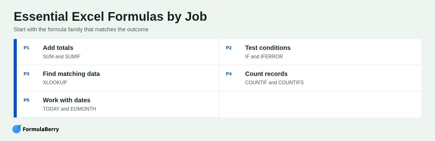
- SUM: Add values. =SUM(B2:B20) totals revenue, expenses, or hours.
- AVERAGE: Find the mean. =AVERAGE(C2:C20) can calculate average order value.
- COUNT: Count numeric cells. =COUNT(D2:D100) counts recorded numeric entries, not text labels.
- MIN: Find the lowest value. =MIN(E2:E50) might identify the smallest invoice amount.
- MAX: Find the highest value. =MAX(E2:E50) finds the largest value in the same range.
- IF: Return one result when a condition is true and another when it is false. =IF(C2>=1000,"Target met","Below target").
- SUMIF: Add values only when they meet a criterion. =SUMIF(A2:A20,"North",B2:B20) totals revenue for the North region.
These are core Excel formulas for calculations because they combine arithmetic with basic decisions. Once you are comfortable with them, the next step is matching records, handling exceptions, and working reliably with dates.
Lookup, cleanup, and date formulas that unlock everyday work
XLOOKUP is the modern starting point for retrieving a matching value from another list. For example, =XLOOKUP(A2,Products!A:A,Products!C:C,"Not found") looks up the product code in A2 and returns its category from column C on the Products sheet. VLOOKUP remains common in legacy workbooks, but XLOOKUP is generally more flexible because the return column does not have to sit to the right of the lookup column.
IFERROR lets you choose what to display when a formula errors. Use it deliberately. =IFERROR(A2/B2,0) may be appropriate when a missing denominator should be treated as zero, but it can also hide a data problem. A blank or a clear message such as "Check input" may be more honest.
COUNTIF and COUNTIFS count records that meet one or multiple conditions. =COUNTIFS(B:B,"Closed",C:C,"North") counts closed deals in the North region. For cleanup, text functions such as TRIM, LEFT, RIGHT, MID, and TEXT help standardize imported data and format values for display.
For date-driven reports, TODAY() returns the current date, while EOMONTH(A2,0) returns the last day of the month containing the date in A2. These are especially useful for aging reports, monthly budgets, and deadline calculations. For more examples, see the Excel Date Formula Guide: Create, Add, Compare, and Fix Dates.
Turn a Plain-English Request into the Right Formula
The quality of formula assistance depends heavily on the quality of the request. Instead of asking, "How do I calculate commission?" turn the work requirement into specific logic that another person, Excel, or an AI formula assistant can interpret consistently.
A reliable request states the output you want, where the inputs are located, the conditions that apply, how missing data should behave, and the Excel version if compatibility matters.
Write a useful formula request
Include the sheet or table name, column names, result type, criteria, date rules, blank handling, error handling, and a sample row whenever possible. This eliminates much of the back-and-forth caused by vague requirements.
A weak request might be: "Create a formula for a discount."
A stronger request might be: "In Sales!G2, return the discounted total. Multiply Revenue in E2 by 90% when Customer Type in C2 is 'Member'; otherwise return Revenue. If Revenue is blank, return blank. The formula will be copied down through row 500."
The stronger version tells you the destination, the inputs, the condition, the expected fallback, and how the formula will be used. It also makes testing straightforward.
Validate a suggested formula before filling it down
Never paste a generated formula into a production range without checking it first. Put it into one test row and compare the result with a hand-calculated expected value.
- Confirm that relative and absolute references move or stay fixed as intended.
- Test a normal case, a zero value, a blank input, and a no-match case.
- Check that criteria text matches the actual data, including spaces and spelling.
- Copy the formula to a few rows before applying it to the full dataset.
- Inspect the formula bar in each test row, not just the displayed output.
As covered in the section on references, a formula can pass its first-row test yet fail when copied if a lookup range or rate cell was not locked correctly.
Use AI for Excel Formula Assistance Without Losing Control
AI formula assistance is most useful when you need a first draft from a business description, a plain-language explanation of a long formula, or help identifying likely logic mistakes. It can reduce the time spent translating requirements into Excel syntax, especially for users who do not work with formulas every day.
It does not replace review. An AI tool does not automatically know your workbook's real structure, the meaning of your fields, or the internal policy behind a calculation unless you provide that context. Share only the necessary schema and sample values, and avoid exposing sensitive customer, financial, or employee data when it is not needed to describe the formula task.
FormulaBerry for formula generation, explanation, and correction
FormulaBerry is a formula assistant for Microsoft Excel and Google Sheets that can generate, explain, and help correct formulas from natural-language requests. It is useful when the hard part is expressing a requirement in formula terms rather than simply locating a function in Excel's menus.
For a useful result, provide the column meanings, desired output, conditions, expected behavior for blanks or missing matches, and at least one sample row. For example: "Revenue is in E2, deal status is in B2, and region is in C2. Return commission only for Closed deals; use a region rate lookup; return blank when revenue is blank."
Use the result as a starting point, then validate it in the actual workbook with the test cases described earlier. Formula generation is not a substitute for confirming that the referenced ranges, business rules, and edge-case behavior are correct.
Copilot in Excel for workbook-aware assistance
When available in your version of Excel, Copilot can provide in-app assistance with workbook-related tasks, including formula and analysis questions. Its main potential advantage is context: it may work with the workbook environment rather than relying only on a text description you provide elsewhere.
Feature availability can depend on your Microsoft 365 plan, region, organization settings, and Excel version. Review generated formulas just as carefully as any other suggestion, particularly when calculations influence financial reporting, operational decisions, or external reporting.
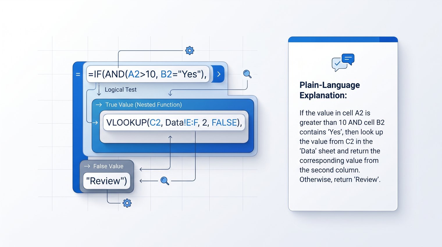
Understand Any Excel Formula, Including Nested Formulas
Long formulas become manageable when you stop trying to read them left to right in one pass. The practical approach is to identify the final action first, then unpack the pieces supplying information to that action.
Read from the outside in
Consider this formula:
=IFERROR(XLOOKUP(A2,Products!A:A,Products!C:C),"Not found")
The outer function is IFERROR. Its job is to return the normal result if the inner formula works, or "Not found" if the inner formula returns an error. The inner formula is XLOOKUP, which searches for the value in A2 within Products column A and returns the matching value from Products column C.
Translated into plain English: "Find the product associated with the code in A2. If no matching product can be found, display Not found instead of an error."
This outside-in method works for nested IF statements, text cleanup, date logic, and lookup formulas. Identify the outer function, list its arguments, and then decode any argument that is itself a formula. Do not skip the references: they often reveal more about the formula's true purpose than the function names do.
Use named ranges, helper cells, and LET to make formulas readable
Sometimes the best way to understand a formula is to refactor it. A single dense formula may be technically correct but difficult to audit, update, or hand off to a colleague.
Named ranges replace vague addresses with meaningful labels. A formula using CommissionRate is easier to review than one using $J$2:$J$10. Helper cells split a complicated calculation into visible steps, which is often the right choice when transparency matters more than compactness.
Modern Excel also supports LET, which lets you assign a name to a repeated value or calculation within a formula. For example:
=LET(net,E2-F2,IF(net>0,net*G2,0))
Here, Excel calculates E2-F2 once, calls the result net, and then uses that name in the condition and calculation. This reduces repetition and makes the logic easier to inspect.
Diagnose Excel Formula Errors Systematically
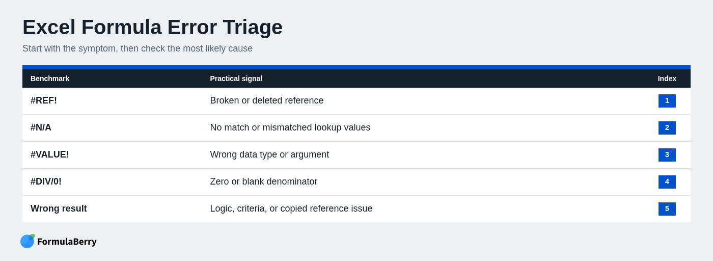
Trial-and-error editing is slow and risky. Start with the symptom, identify the likely cause, and check the relevant cells before changing the formula. This applies both to visible Excel errors and to formulas that return a plausible but wrong answer.
What common Excel errors mean
- #VALUE! usually means Excel received the wrong data type or argument, such as text where a number is expected. Check the referenced cells for text, hidden characters, or incompatible ranges.
- #N/A usually means a lookup did not find a match. Confirm that lookup values use the same spelling, data type, and formatting on both sides.
- #REF! means a reference is broken, often because a referenced cell, row, column, or sheet was deleted.
- #DIV/0! means a formula is dividing by zero or by a blank cell. Inspect the denominator and decide what the intended fallback should be.
- #NAME? means Excel does not recognize text in the formula, often because a function was misspelled or text was not enclosed in quotation marks.
- #NUM! indicates an invalid numeric calculation, such as an impossible number argument or a calculation Excel cannot resolve.
- #### often means the column is too narrow to display the value. With dates or times, it can also indicate a negative date or time result. It is not automatically evidence of a broken formula.
When the formula works but the answer is wrong
The more dangerous spreadsheet problem is a valid formula that returns an incorrect result without any error code. Start by checking whether numbers are stored as text, whether imported values contain hidden spaces, and whether criteria text exactly matches the source data.
Dates deserve special attention. Excel stores valid dates as serial values, but imported dates may be text strings that only look like dates. Also check calculation mode, particularly if a workbook appears not to recalculate after changes. A copied formula may have reference drift, where a range shifts unexpectedly because it was relative rather than absolute.
When someone says an "Excel formula is not working," separate the problem into two categories: an error value that Excel can identify, or a wrong-but-valid output caused by logic, data, or references. The troubleshooting path is different for each.
Use Excel's Formula Auditing Tools to Find the Breakpoint
Formula auditing tools help you investigate complex calculations without rewriting the workbook. They are particularly useful when a formula is used across many rows or pulls inputs from several sheets.
Trace Precedents, Trace Dependents, and Error Checking
Trace Precedents shows the cells that feed into the selected formula. Use it when you need to find an upstream input that may be wrong. Trace Dependents shows formulas that rely on the selected cell, which is helpful before changing a rate, assumption, or key calculation.
Error Checking guides you through identified formula errors and can help navigate to the cells involved. It is useful for obvious error values, but it will not detect every logic problem. A formula returning the wrong number may require a closer review of the criteria and references.
After investigating, remove visual arrows using Excel's Remove Arrows command so the worksheet remains readable.
Evaluate Formula and Watch Window
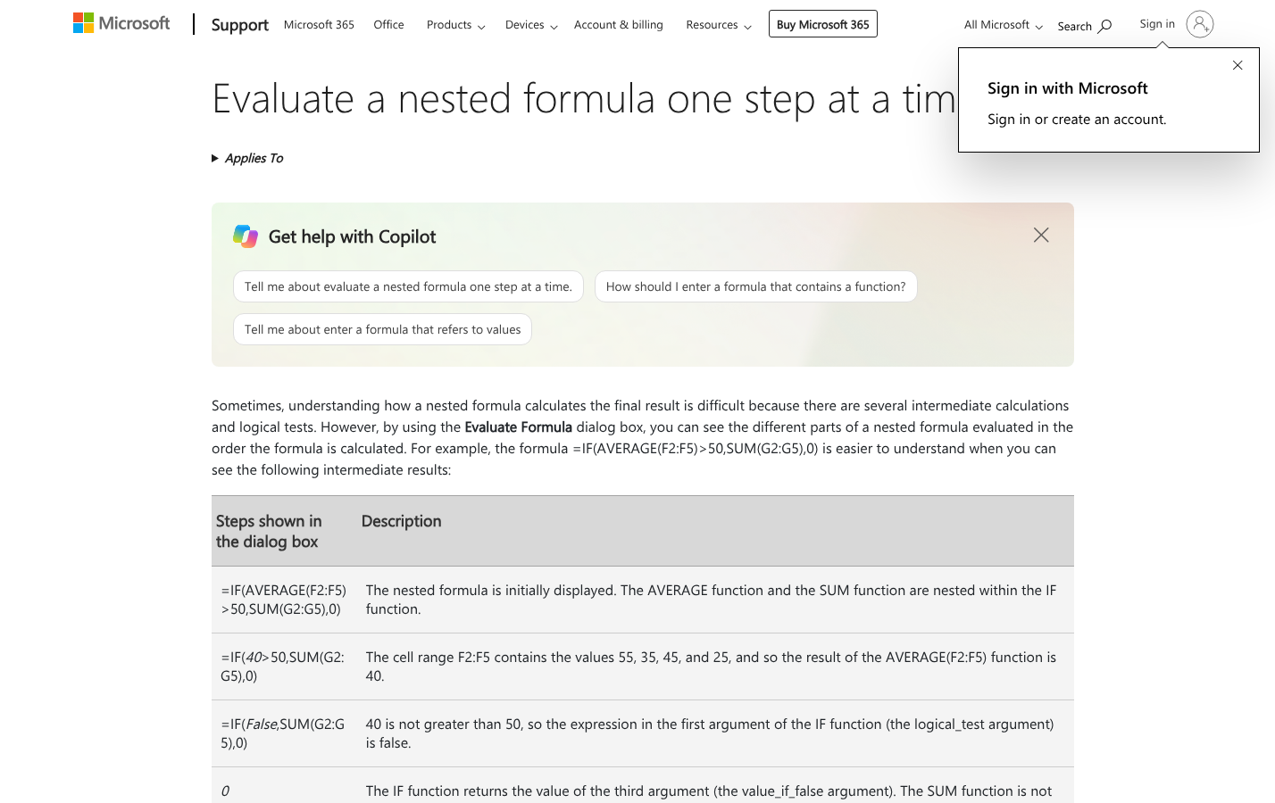
Evaluate Formula reveals intermediate calculation steps one at a time. This is one of the most reliable ways to understand where a nested IF, lookup, or text-cleaning formula changes from expected to unexpected. Instead of guessing which piece is responsible, you can watch Excel calculate each segment.
Watch Window is useful when troubleshooting across sheets. Add important cells to the watch list and monitor their values and formulas while you inspect inputs elsewhere in the workbook. It is especially practical for models with assumptions on one sheet and calculations on another.
Fix Inconsistent Formulas Before They Spread
An inconsistent formula is a formula that breaks the surrounding pattern. Excel may flag this with an inconsistent formula warning, but a difference is not automatically an error. The row could contain an intentional exception, such as a special discount or a manually approved adjustment.
The correct response is to verify the pattern before accepting a suggested correction. Do not overwrite a legitimate exception merely because it differs from nearby rows.
Compare the formula pattern, not just the displayed value
Values can look reasonable even when formulas differ. Compare the formulas in adjacent rows through the formula bar or switch to formula view to see the pattern across a range.
Look for shifted ranges, missing criteria, changed sheet references, and hard-coded values where a cell reference should appear. A disciplined row-by-row comparison is often faster than trying to infer the problem from totals alone.
Use tables and structured references to prevent copy errors
Excel Tables help prevent copy-down mistakes because calculated columns apply a consistent formula pattern. Structured references also make logic clearer. For example, =IF([@Status]="Closed",[@Revenue]*[@Rate],"") communicates the purpose of each input better than a formula containing only cell coordinates.
Tables are not a cure for every issue. Review row-level overrides and exceptions, and confirm that a table formula still reflects the intended rule when columns are added, renamed, or repurposed.
Worked Example: Build, Explain, and Repair a Commission Formula
Suppose a sales team needs a commission calculation. Commission should be paid only on closed deals. The rate depends on the deal's region. Incomplete revenue should return a blank, and a missing region in the rate table should be visible rather than silently treated as zero.
Step 1: translate the business rule into testable logic
Assume the Deals table has these columns: Status, Region, Revenue, and Commission. A separate Rates table has Region and Rate.
Write expected outcomes before entering a formula:
- A Closed deal in North with $10,000 revenue and a 10% rate should return $1,000.
- An Open deal with the same revenue should return 0, because it is not eligible.
- A Closed deal with blank revenue should return blank, because the source record is incomplete.
- A Closed deal in an unmapped region should return "Check rate," not a silent zero.
This step prevents a common mistake: building a technically valid formula that pays commission for open deals or hides missing rate data.
Step 2: build and test the formula
Using table references, one clear formula pattern is:
=IF([@Revenue]="","",IF([@Status]<>"Closed",0,IFERROR([@Revenue]*XLOOKUP([@Region],Rates[Region],Rates[Rate]),"Check rate")))
Read it from the outside in. First, if Revenue is blank, return blank. Next, if Status is not Closed, return 0. Otherwise, look up the region's rate and multiply it by revenue. If the region cannot be found in the Rates table, show "Check rate."
Test the four expected cases. For the North example, the formula should return 1000. For an Open deal, it should return 0. For blank revenue, it should remain blank. For an unknown region, it should display Check rate. Only after those results are correct should you apply the formula across the dataset.
Step 3: repair a broken copied-down version
Now imagine the Rates table is not an Excel Table and is stored in cells J2:K6. A first attempt might use:
=IF(C2="Closed",E2*XLOOKUP(B2,J2:J6,K2:K6),"")
It may work in row 2 but fail after being copied down because J2:J6 and K2:K6 shift to J3:J7 and K3:K7. The fix is to lock the lookup ranges:
=IF(C2="Closed",E2*XLOOKUP(B2,$J$2:$J$6,$K$2:$K$6),"")
If the result is still wrong, select a failing row and use Trace Precedents to confirm the inputs. Then use Evaluate Formula to see whether the failure occurs at the status test, revenue value, lookup, or multiplication step. Once corrected, refill the column carefully and compare several rows against independent hand calculations.
Build a Reliable Formula-Checking Habit
Reliable spreadsheet work comes from a repeatable review process, not from trusting a formula because it looks sophisticated. Before treating a calculation as final, check the inputs, references, criteria, error behavior, edge cases, and fill pattern.
- Are source values complete and stored in the correct data type?
- Do absolute and relative references behave correctly when copied?
- Do criteria match the values actually used in the sheet?
- What should happen for blanks, zeroes, missing matches, and errors?
- Have you tested a few rows with independently calculated expected results?
- Is the logic documented through clear headers, named ranges, helper cells, or notes?
Keep business logic separate from raw imported data where practical. A dedicated assumptions or rates table is easier to review than constants hidden inside dozens of formulas. Descriptive headers and named ranges also make formulas far easier for another person to audit later.
Before you share or publish a workbook
Check that calculation mode is appropriate and that key formulas have recalculated. Search for error cells, inspect for formulas accidentally overwritten by hard-coded values, and review any constants embedded in formulas that should instead come from an assumptions table.
Reconcile important totals to an independent calculation whenever possible. For high-stakes financial, operational, or reporting workbooks, a second reviewer should inspect the logic and a representative sample of source records. A peer review is often much cheaper than correcting a decision made from a bad spreadsheet.
Get Faster, More Reliable Help with Excel Formulas
Good Excel formula assistance follows a simple progression: use Excel's built-in guidance while entering formulas, use auditing tools when results need investigation, and describe the requirement clearly when the logic itself is difficult to translate.
Start with a small test, validate references and edge cases, then fill the formula across the real range. When you need to create, explain, or correct a formula from a plain-English request, FormulaBerry can help you get to a workable formula faster - then validate that result against the actual workbook and business rule.