Excel text cleanup gets frustrating when the value you need sits in the middle of a code, reference, or imported field. A simple copy-and-paste approach may work once, but it breaks down fast when you have hundreds of rows.

The Excel MID formula solves that problem by extracting characters from a specific position. It can pull a fixed segment from a structured ID or, when combined with FIND, return text located between delimiters such as hyphens, underscores, and parentheses.

How the Excel MID function works

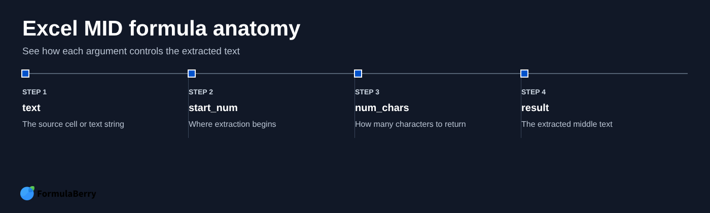
MID is a text function that returns a chosen number of characters starting at a specified position in a cell or text string.

The syntax is:

=MID(text, start_num, num_chars)

• text is the source text or cell reference to read from.
• start_num is the character position where extraction begins.
• num_chars is the number of characters Excel should return.

For example, this formula returns the five-digit number from an invoice reference:

=MID("INV-48291-US",5,5)

The result is 48291. Excel starts at character 5, which is the first digit after INV-, then returns five characters.

Extract a fixed number of characters from the middle of a cell

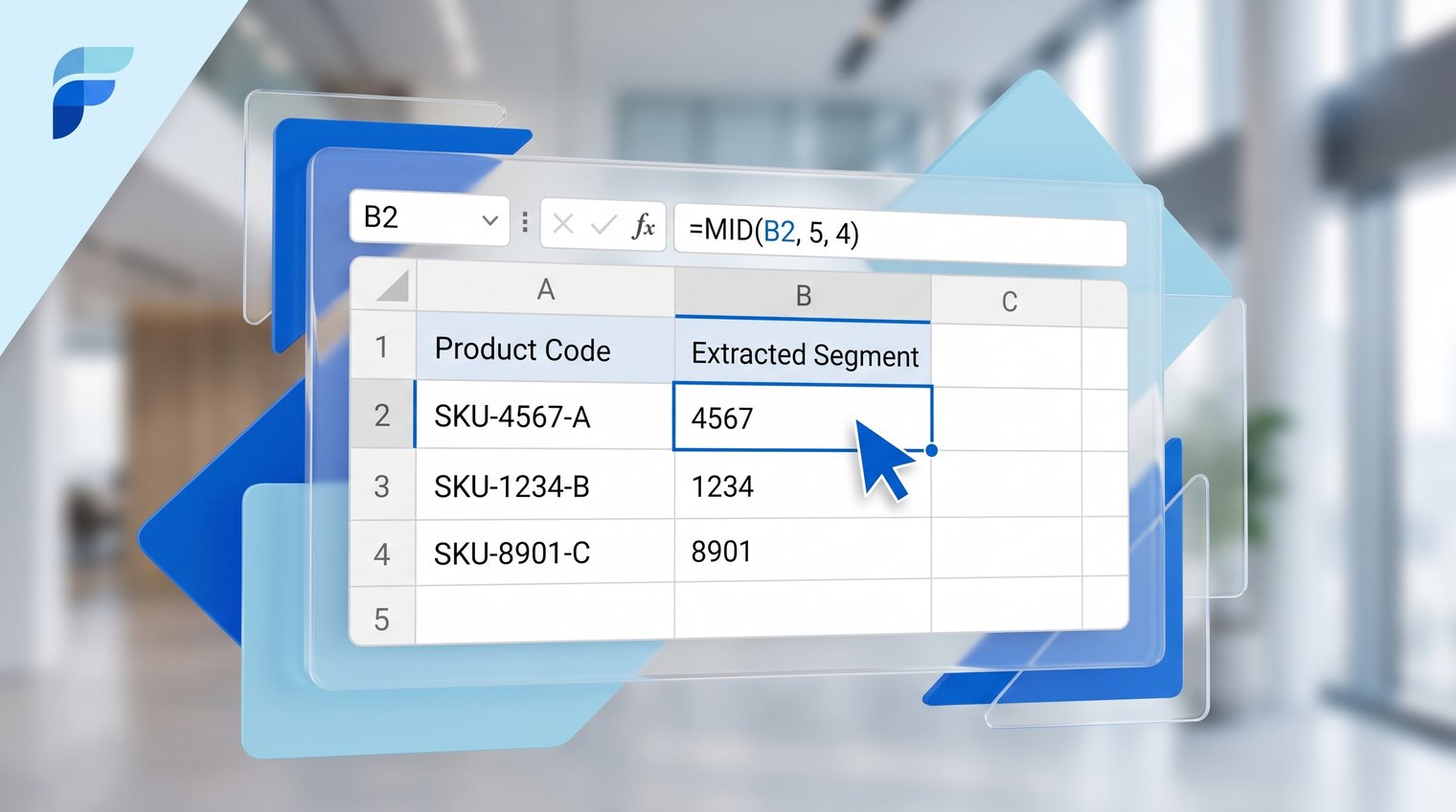
The most straightforward MID formula uses a cell reference and known positions. If product codes in column A always follow the pattern PRD-48291-US, use:

=MID(A2,5,5)

With PRD-48291-US in A2, the formula returns 48291. The fifth character is the first character after the prefix and hyphen, and the middle code is always five characters long.

Count every character when identifying the start position. Spaces, hyphens, slashes, periods, and parentheses all count. In PRD-48291-US, the characters are:

• P = 1
• R = 2
• D = 3
• - = 4
• 4 = 5

Enter the formula in the first result cell, then drag the fill handle down the column. Excel adjusts A2 to A3, A4, and so on automatically.

Common mistake: Do not start counting after the first hyphen unless you account for it in the formula. MID counts from the beginning of the entire cell, not from a separator.

Use MID to extract text between two characters

Fixed positions are useful only when every row follows the same format. If the middle segment can vary in length, locate its surrounding delimiters first.

For values separated by two hyphens, this reusable formula finds the text between them:

=MID(A2,FIND("-",A2)+1,FIND("-",A2,FIND("-",A2)+1)-FIND("-",A2)-1)

It looks complicated because it does two jobs: it finds where the first hyphen is, then finds where the next hyphen is. MID starts one character after the first hyphen and extracts everything before the second one.

Extract text between the first and second hyphen

Suppose A2 contains:

Region-East-2026

Use:

=MID(A2,FIND("-",A2)+1,FIND("-",A2,FIND("-",A2)+1)-FIND("-",A2)-1)

The result is East.

The first FIND("-",A2) returns the position of the first hyphen. The second FIND starts searching one character after that first hyphen:

FIND("-",A2,FIND("-",A2)+1)

That starting point matters. Without it, Excel would locate the first hyphen twice, leaving MID with an invalid length calculation.

Adapt the formula for other delimiters

You can replace the hyphen in the formula with another separator. For example, use "/" for slash-separated values, "_" for underscore-separated text, or parentheses when a value appears in brackets.

For Sales/West/2026, replace each hyphen with a slash:

=MID(A2,FIND("/",A2)+1,FIND("/",A2,FIND("/",A2)+1)-FIND("/",A2)-1)

If you need Excel to ignore letter case while finding text rather than punctuation, use SEARCH instead of FIND. FIND is case-sensitive; SEARCH is not.

Extract a variable-length value with MID

A hard-coded character count fails as soon as the text between separators changes length. For example, both of these values have the same structure but very different color names:

• SKU-RED-XL
• SKU-MIDNIGHTBLUE-XL

If you use =MID(A2,5,3), it returns RED correctly from the first value. But it returns only MID from the second. The problem is not MID itself; the problem is telling it to return a fixed three-character result.

Instead, calculate the number of characters between the first and second hyphens:

=MID(A2,FIND("-",A2)+1,FIND("-",A2,FIND("-",A2)+1)-FIND("-",A2)-1)

This returns RED for the first SKU and MIDNIGHTBLUE for the second. The formula adapts because the third MID argument is calculated from the delimiter positions.

Use this approach whenever the segment begins and ends with recognizable markers but has an inconsistent length across rows.

Combine MID with LEFT and RIGHT for text cleanup

LEFT, RIGHT, and MID all extract characters, but they work from different locations. LEFT starts at the beginning of a value, RIGHT starts at the end, and MID starts wherever you tell it to start.

With the sample value ORD-48291-US in A2:

• =LEFT(A2,4) returns ORD-.
• =RIGHT(A2,2) returns US.
• =MID(A2,5,5) returns 48291.

These functions are not interchangeable. Choose the one that matches where the required value sits.

Choose MID when the value is not anchored to an edge

Use MID when the target is in the center of a cell, particularly when you know its start position and length. A sales reference such as ORD-48291-US has a prefix on the left and country code on the right, so MID is the right function for the order number.

Modern Excel functions can make delimiter-based extraction easier in some cases, but MID remains a dependable choice for fixed-position fields and workbooks shared with people using older versions of Excel.

Use MID to pull date parts stored as text

MID can extract portions of a date only when the date is stored as text. If Excel recognizes a value as a real date, use date functions such as MONTH, YEAR, and DAY instead.

For text in the format YYYY-MM-DD, such as 2026-04-18 in A2, extract the month with:

=MID(A2,6,2)

The result is 04. The month starts at character 6 because the fifth character is the first hyphen.

To turn text date components into a usable Excel date, combine DATE and VALUE:

=DATE(VALUE(LEFT(A2,4)),VALUE(MID(A2,6,2)),VALUE(RIGHT(A2,2)))

This creates a real date value from a text string in the YYYY-MM-DD format. You can then sort it, filter it, or use it in date calculations. For additional formatting options after conversion, see the Excel TEXT formula guide.

Handle errors and inconsistent source text

Delimiter-based formulas assume the expected separators exist. If a row is missing a hyphen, contains an extra hyphen, or uses a different pattern, FIND may return an error.

Before filling a formula down thousands of rows, inspect a sample from the top, middle, and bottom of the source column. Look specifically for blanks, malformed entries, extra spaces, and alternate formats.

When a blank result is appropriate for invalid rows, wrap the formula in IFERROR:

=IFERROR(MID(A2,FIND("-",A2)+1,FIND("-",A2,FIND("-",A2)+1)-FIND("-",A2)-1),"")

This prevents #VALUE! from appearing when a required hyphen is missing. A blank is useful when incomplete rows are expected and will be reviewed later. If bad input needs immediate attention, return a visible flag instead:

=IFERROR(MID(A2,FIND("-",A2)+1,FIND("-",A2,FIND("-",A2)+1)-FIND("-",A2)-1),"CHECK FORMAT")

Why MID returns an unexpected result

Most unexpected MID results come from off-by-one counting. A separator occupies a character position, so start after it by adding 1 to the FIND result.

Another issue is finding the wrong occurrence of a delimiter. When a value contains more than one hyphen, a second FIND must begin after the first result; otherwise, Excel repeatedly identifies the same separator.

MID does not always generate an error when num_chars is too large. If the requested length extends past the end of the text, Excel typically returns the characters that remain. For example, =MID("ABC",2,10) returns BC.

Use modern Excel alternatives when they are clearer

Microsoft 365 users may have access to TEXTBEFORE, TEXTAFTER, and TEXTSPLIT. These functions often make delimiter-based extraction easier to read than a nested FIND and MID formula.

For example, to return East from Region-East-2026, you can use:

=TEXTBEFORE(TEXTAFTER(A2,"-"),"-")

The inner TEXTAFTER removes everything through the first hyphen. TEXTBEFORE then returns everything before the next hyphen.

MID is still the better default for exact positions, legacy workbook compatibility, and situations where the source format is based on character locations rather than delimiters.

MID versus TEXTBEFORE and TEXTAFTER

For text between two hyphens, TEXTAFTER and TEXTBEFORE are more readable when your Excel version supports them. MID with FIND is more broadly compatible and gives you precise control over the starting position and returned character count.

Check who will open the workbook before adopting newer functions. A formula that works perfectly in your Microsoft 365 desktop app may not work for a colleague using an older Excel release.

Check MID formulas quickly with an AI formula assistant

When a source column has an unusual pattern, describe the actual value, the intended result, and any exceptions before asking for a formula. For example: "In A2, extract the text between the first and second hyphen. Return blank if either hyphen is missing."

Then test the resulting formula against normal rows and edge cases, including missing separators, longer segments, and unexpected extra delimiters. Formula generation is faster when the request is specific, but validation is still your responsibility.

FormulaBerry

FormulaBerry can generate, explain, and help correct formulas for Excel and Google Sheets from a plain-language request. It is particularly useful when you understand the desired output but do not want to manually construct nested FIND, IFERROR, and MID logic.

It is a formula assistant, not a full spreadsheet application or automatic data-cleaning system. You still need to provide a representative cell pattern and confirm the result in your workbook. Choose it when you need help translating a business rule into a formula or diagnosing why an existing formula is returning the wrong segment.

Excel MID formula examples to keep handy

Task	Sample input in A2	Formula	Result
Fixed-position extraction	PRD-48291-US	=MID(A2,5,5)	48291
Text between two hyphens	Region-East-2026	=MID(A2,FIND("-",A2)+1,FIND("-",A2,FIND("-",A2)+1)-FIND("-",A2)-1)	East
Variable-length SKU segment	SKU-MIDNIGHTBLUE-XL	=MID(A2,FIND("-",A2)+1,FIND("-",A2,FIND("-",A2)+1)-FIND("-",A2)-1)	MIDNIGHTBLUE
Month from a text date	2026-04-18	=MID(A2,6,2)	04

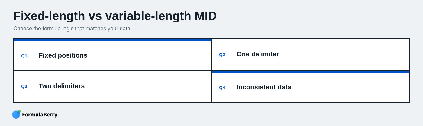
Use the fixed-position formula when every value follows the same character layout. Use the delimiter-based formula when the middle segment can vary in length. Use the date example only when the date is text rather than a true Excel date value.

Extract the exact text segment you need with MID

MID is the practical choice when you know where the needed text starts and how many characters to return. When positions vary, pair MID with FIND or SEARCH so the formula calculates the start and length from the separators in each row.

For real-world data, build in error handling before you fill a formula down, especially when imported files may contain blanks or inconsistent formats. If you need help building or debugging a formula for your own cell pattern, FormulaBerry can turn a clear plain-language requirement into a starting formula you can test in Excel or Google Sheets.