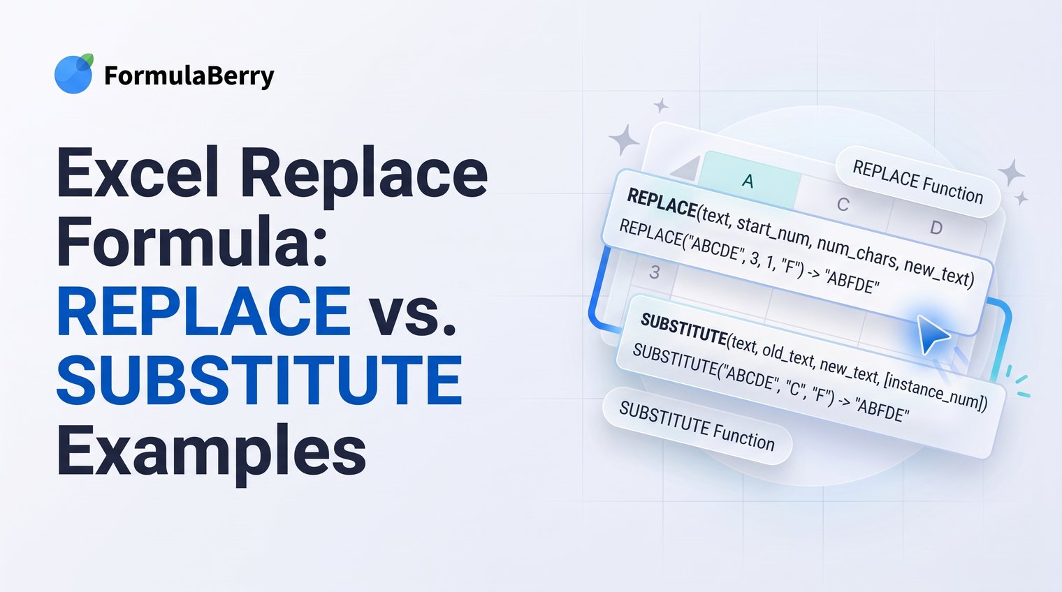
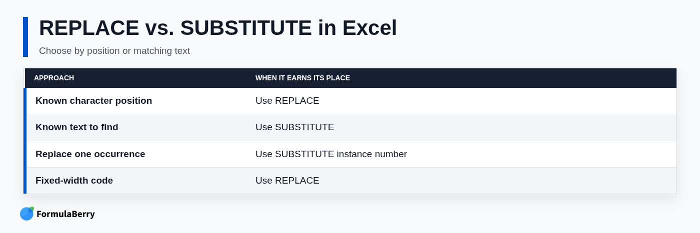
Excel text replacements go wrong when you choose the function based on its name instead of the structure of your data. If you know where the characters sit, use REPLACE. If you know which text you want to change, use SUBSTITUTE.

That distinction handles most Excel replace formula tasks. For example, =REPLACE("555-123-4567",5,3,"999") changes characters 5 through 7, while =SUBSTITUTE("A-B-C","-","/") changes every hyphen it finds.

Choose the right Excel replace formula first

Use REPLACE when the part to change is always in a known character position. It does not check what the existing characters are; it simply starts at a position you specify and overwrites a set number of characters.

Use SUBSTITUTE when you need Excel to find matching text, such as a hyphen, old email domain, word, or code prefix. It replaces matching text wherever it appears, or at one specific occurrence if you tell it which one.

• Known position: =REPLACE(A2,1,3,"EU-")
• Known text: =SUBSTITUTE(A2,"-","/")

A product code with a fixed three-character prefix is usually a REPLACE job. A list of inconsistent values containing hyphens, spaces, or an outdated company name is usually a SUBSTITUTE job.

Use REPLACE when the characters are in a known position

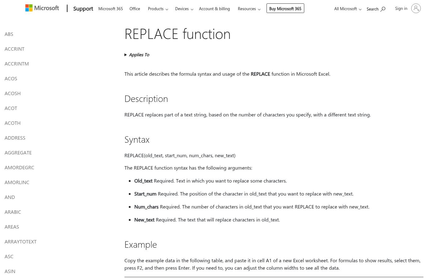
REPLACE changes a specified number of characters starting at a specified position. Its syntax is:

=REPLACE(old_text, start_num, num_chars, new_text)

• old_text is the original cell value or text string.
• start_num is the character position where replacement begins.
• num_chars is how many existing characters Excel removes.
• new_text is the replacement text you want to insert.

Excel counts positions from 1, not 0. REPLACE works with text strings, including numbers that are stored as text. That matters for IDs, account references, postal codes, and other values where leading zeros must remain intact.

REPLACE syntax, a simple phone-number example, and a Microsoft Support reference

Suppose you need to change the middle three digits of a phone number:

=REPLACE("555-123-4567",5,3,"999")

The result is 555-999-4567. Position 5 is the first character in 123, and Excel replaces three characters beginning there. The hyphens remain because they are outside the three-character replacement range.

For a cell reference, use the same pattern:

=REPLACE(A2,5,3,"999")

The important detail is that REPLACE does not search for 123. If the value at positions 5 through 7 changes to another three characters, Excel will still replace that same location.

Replace a fixed part of an ID or product code

Imagine column A contains product codes such as US-10492, CA-20418, and JP-77201. If the first three characters should become EU-, use:

=REPLACE(A2,1,3,"EU-")

If A2 contains US-10492, the result is EU-10492. This is safer than SUBSTITUTE when the first three characters may vary but their position and length are fixed.

Keep identifiers formatted as text when leading zeros matter. For example, an ID such as 001245 can lose zeros if Excel treats it as a number before your formula has a chance to work with it.

Use SUBSTITUTE when you need to find and replace text

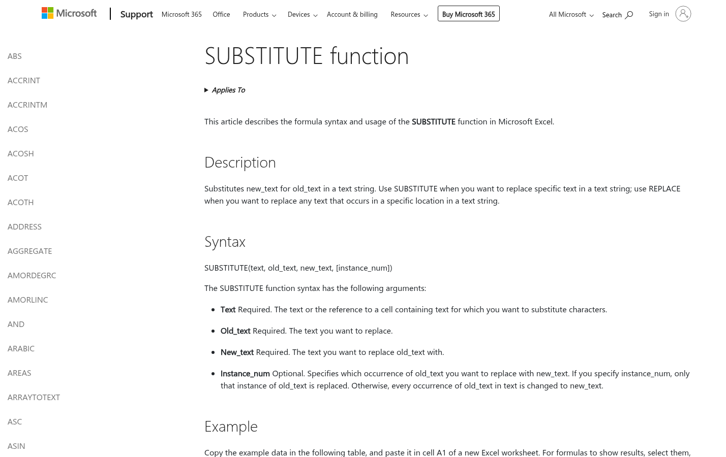
SUBSTITUTE is the better Excel replace text formula when you know the exact characters or word to change but do not want to count its position. By default, it replaces every exact match in the text.

The syntax is:

=SUBSTITUTE(text, old_text, new_text, [instance_num])

• text is the original cell value or text string.
• old_text is the text Excel should find.
• new_text is the text that replaces it.
• instance_num is optional and lets you change only one occurrence.

Use SUBSTITUTE to find and replace a character in an Excel formula, such as swapping hyphens for slashes, removing spaces, or replacing an old email domain.

SUBSTITUTE syntax, an all-occurrences example, and a Microsoft Support reference

If A2 contains 2026-09-16 and you want slashes instead of hyphens, enter:

=SUBSTITUTE(A2,"-","/")

The result is 2026/09/16. Because no instance number is supplied, Excel replaces every hyphen it finds. If you need to build, compare, or troubleshoot dates rather than replace their display characters, see this Excel Date Formula Guide.

SUBSTITUTE is case-sensitive. Searching for "sku" will not replace "SKU". This can explain why a formula appears to do nothing even though the text looks similar at a glance.

Replace only the second or third occurrence

To change one specific match, add the optional fourth argument. For example:

=SUBSTITUTE("A-B-C-D","-","/",2)

The result is A-B/C-D. Excel finds the second hyphen only and changes it to a slash.

Without the final 2, all three hyphens would be replaced. If you request an occurrence that does not exist, SUBSTITUTE returns the original text unchanged. That is useful in some cleanup workflows, but it can also conceal inconsistent source data, so verify a sample of your results.

Work through common Excel replace formula examples

The fastest way to get comfortable with these functions is to apply them to real cell values. Put formulas in a helper column first so you can compare the original value with the cleaned result.

Remove unwanted characters with SUBSTITUTE

To remove ordinary spaces from the value in A2, replace them with an empty text string:

=SUBSTITUTE(A2," ","")

If A2 contains AB 123 45, the result is AB12345. The two quotation marks at the end mean "replace with nothing."

A common mistake is assuming every visible space is an ordinary keyboard space. Data copied from websites or exported from another system may contain nonbreaking spaces. For those, use:

=SUBSTITUTE(A2,CHAR(160),"")

If a normal space formula does not remove a visible gap, CHAR(160) is the first fix worth trying.

Replace an email domain without changing the username

If A2 contains maria@oldcompany.com, this formula updates only the domain:

=SUBSTITUTE(A2,"@oldcompany.com","@newcompany.com")

The result is maria@newcompany.com. Matching the complete domain, including the @ sign, is more precise than replacing just oldcompany, which could appear elsewhere in a value.

This pattern is especially useful when you need a repeatable transformation for a contact export rather than a one-off edit to a few cells.

Mask part of a value while keeping its format

If every account reference begins with six characters that should be hidden, use:

=REPLACE(A2,1,6,"XXXXXX")

For an input of 123456-7890, the result is XXXXXX-7890. The original layout remains because the hyphen and final digits are not touched.

Only use this approach when the mask location is genuinely consistent. If some account values have different prefix lengths, calculate the delimiter position first instead of assuming six characters in every row.

Replace text after a delimiter when the position varies

REPLACE becomes more flexible when you pair it with FIND. FIND identifies the position of a delimiter, such as a hyphen, so the formula can adapt to values of different lengths.

Replace everything before a hyphen

For values such as OLD-1042, replace the text before the hyphen with:

=REPLACE(A2,1,FIND("-",A2)-1,"NEW")

The result is NEW-1042. FIND returns the position of the hyphen. Subtracting 1 tells REPLACE to stop just before it, preserving the delimiter.

For example, in OLD-1042, the hyphen is character 4. REPLACE starts at character 1 and changes the first three characters, OLD, to NEW.

Replace everything after a hyphen

To keep the prefix and replace everything after the hyphen, use:

=REPLACE(A2,FIND("-",A2)+1,LEN(A2),"ARCHIVED")

If A2 contains OLD-1042, the result is OLD-ARCHIVED. The formula starts one character after the hyphen, then replaces the rest of the string.

REPLACE can use a character count larger than the remaining text, so using LEN(A2) is a simple reliable default. If some cells do not contain a hyphen, FIND returns an error. In that case, wrap the formula with IFERROR:

=IFERROR(REPLACE(A2,FIND("-",A2)+1,LEN(A2),"ARCHIVED"),A2)

That version leaves values without a hyphen unchanged.

Avoid the mistakes that cause incorrect replacements

Most replacement errors come from source data inconsistencies or incorrect character counts, not from a complicated formula. Check the value in the source cell before changing the formula repeatedly.

Check positions, character counts, and hidden spaces

REPLACE uses exact character positions. An off-by-one error can remove a delimiter you meant to keep, or leave behind one character from the old text. Count from the first character as position 1, and decide explicitly whether a hyphen, slash, or space should remain in the result.

Use =LEN(A2) to check the total character count when a value appears suspicious. Extra spaces at the beginning or end of a cell are easy to miss, and nonbreaking spaces are different from ordinary spaces.

For example, if you want to retain a hyphen in OLD-1042, your replacement length should end at the character before the hyphen. Replacing through the hyphen requires adding the new delimiter back into your replacement text.

Handle missing text and case differences

SUBSTITUTE returns the original value when it cannot find an exact match. That can be desirable, but do not interpret an unchanged result as proof that the data was already correct. It may use a different case, contain a hidden space, or have a slightly different spelling.

Remember that SUBSTITUTE is case-sensitive. If your values include both SKU-100 and sku-100, a formula that searches for one version will not change the other.

FIND-based formulas behave differently: FIND produces an error when the delimiter is missing. Use IFERROR when missing delimiters are expected, or filter and correct those inconsistent records before applying the formula.

Know when Find and Replace is better than a formula

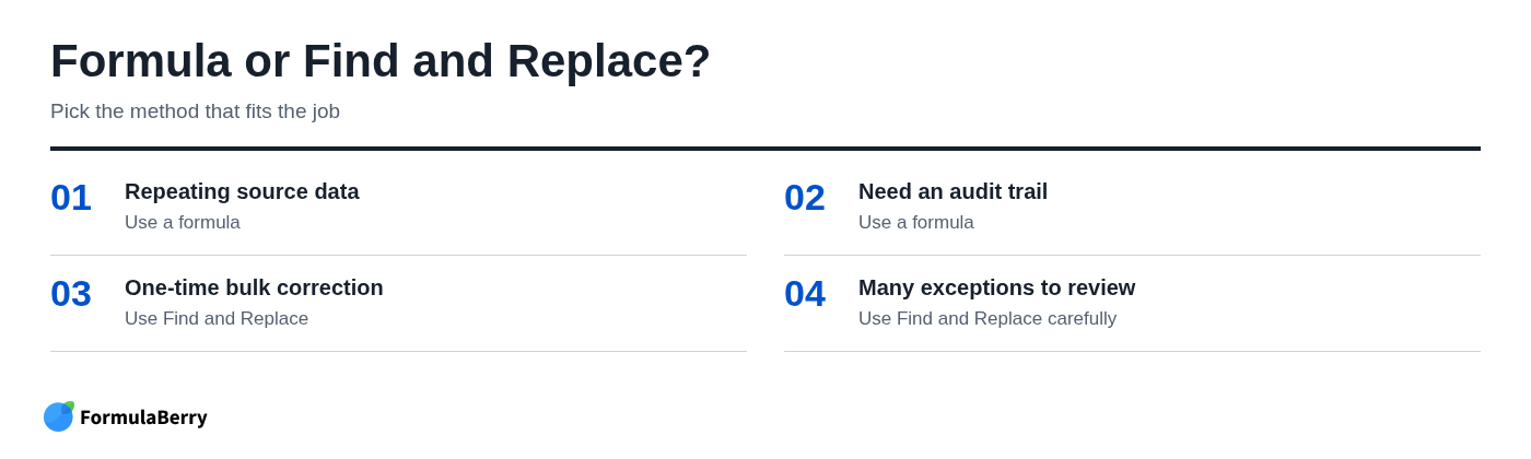
Excel's Find and Replace command is useful for a one-time bulk correction in selected cells. If you need to fix one typo across a finished worksheet and do not need to preserve the original values, it may be the quickest option.

Use a formula when the transformation needs to be repeatable, reviewable, or updated as source data changes. A helper column using REPLACE or SUBSTITUTE keeps the raw value intact and recalculates automatically when A2 changes.

• Repeating source data: use a formula.
• Need to compare old and new values: use a formula.
• One-time bulk correction: Find and Replace may be faster.
• Many exceptions to inspect: review carefully before replacing values permanently.

Do not overwrite operational IDs, customer data, or imported records before validating several formula results. Once you are confident, you can copy the formula output and use Paste Values in a final column if static results are required.

Apply the formula down a column and preserve the original data

Start by keeping the original values in column A and placing your replacement formula in column B. For example, enter =SUBSTITUTE(A2,"-","/") in B2, then check several rows with short, long, and unusual values before filling the formula down.

In a standard range, drag the fill handle from the lower-right corner of the formula cell, or double-click it when the adjacent data column is continuous. In an Excel Table, entering the formula once typically fills the entire calculated column automatically and continues as new rows are added.

If the formula output will become the final operational value, make a copy of the workbook first. After checking the results, copy the helper column and paste values where needed. This preserves the transformed text without leaving formulas tied to the original source column.

Use REPLACE for positions and SUBSTITUTE for matches

The decision rule is simple: use REPLACE when you know the character location to overwrite, and use SUBSTITUTE when you know the text Excel should find. SUBSTITUTE can replace every match or one selected occurrence; REPLACE is ideal for fixed-width codes, masks, and consistent sections of an identifier.

When the position changes from row to row, combine REPLACE with FIND to locate a delimiter before replacing the relevant part of the value. That gives you a formula-driven process that is easier to review and reuse than manual edits.

If you can describe the spreadsheet change you need but are unsure how to write it, the Excel Formula Generator can help turn a plain-English request into an Excel or Google Sheets formula.