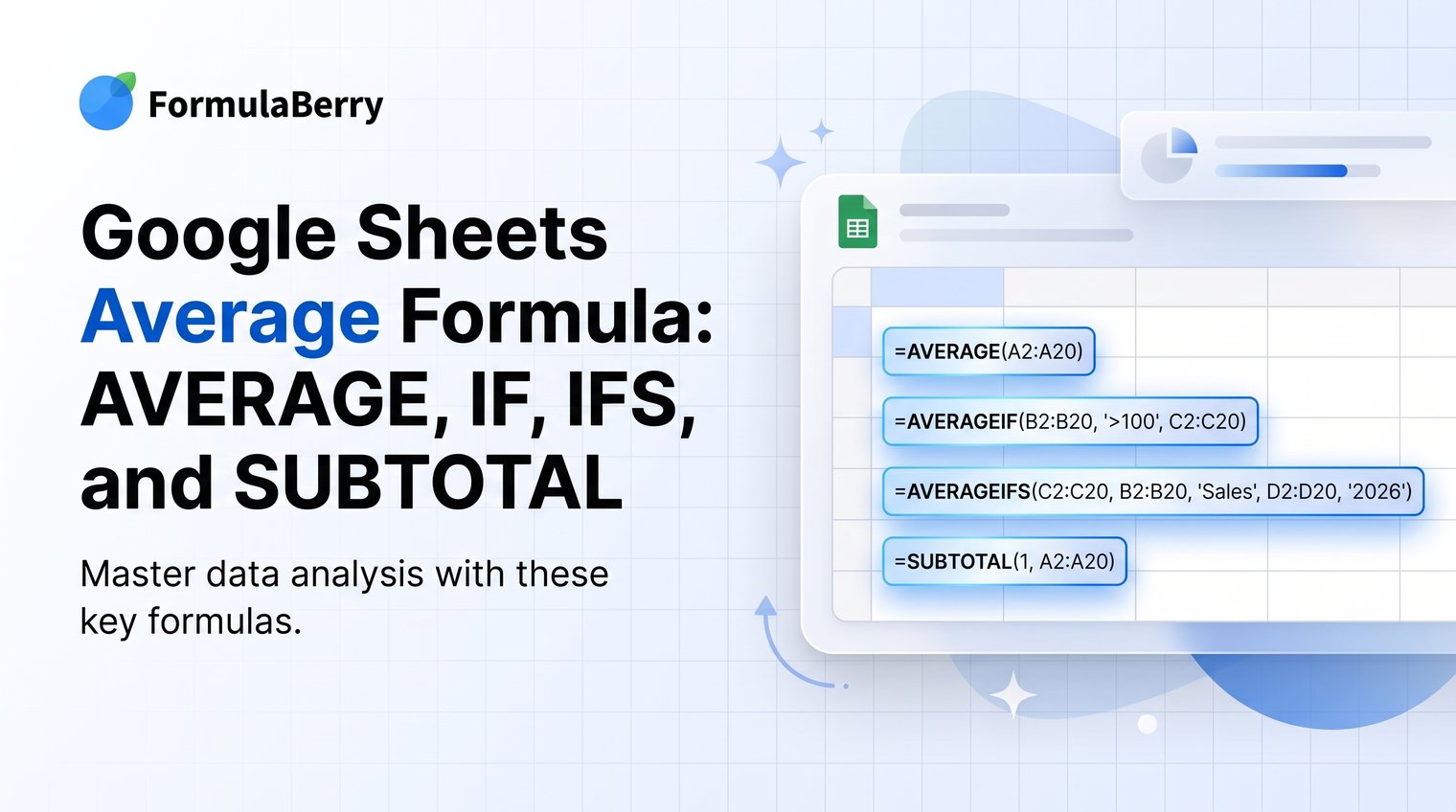
An average can look deceptively simple until your sheet contains blanks, category labels, filters, formula-generated empty cells, and errors. Using AVERAGE on the wrong range can produce a number that is technically correct but useless for the decision you need to make.

This guide shows how to use the Google Sheets average formula for straightforward ranges, conditional averages, and filtered reports. Each formula is copy-ready, so you can adapt it to sales data, grades, budgets, or monthly reporting. If you need help creating or explaining a different formula, see this Google Sheets formula generator.

Use AVERAGE to calculate a simple mean in Google Sheets

For a basic average, use:

=AVERAGE(value1, [value2, ...])

More commonly, average a continuous range of cells:

=AVERAGE(B2:B10)

This formula adds the numeric values in cells B2 through B10 and divides the total by the number of numeric values. If B2:B10 contains 10, 15, and 20, the result is 15.

You can supply individual numbers, cell references, or ranges. For example, all of these are valid:

• =AVERAGE(10,20,30)
• =AVERAGE(B2,B3,B4)
• =AVERAGE(B2:B10)
• =AVERAGE(B2:B10,D2:D10)

In most working sheets, a range reference is the best choice because the formula is easier to read and update.

Average a column, row, or nonadjacent cells

The direction and layout of your data determine the range you use. A column average uses a vertical range, while an average of a row uses a horizontal range.

Average a column

To average values in column C from row 2 to row 100, enter:

=AVERAGE(C2:C100)

You can also average an entire column with:

=AVERAGE(C:C)

That works, but a bounded range is usually clearer. It also reduces the risk of including a future total, manually entered note, or summary formula farther down the column. If row 101 will eventually hold a yearly total, keep your average limited to the data rows instead of averaging the whole column.

Average a row

When monthly values run across columns, use a horizontal range. For example, to average January through December values in row 2:

=AVERAGE(B2:M2)

This is a common Google Sheets formula for an average of a row, especially in budget and performance-tracking templates where each row represents one product, employee, customer, or department.

Average selected, nonadjacent cells

When the values you need are separated, list the references individually:

=AVERAGE(B2,B5,B9)

You can also combine multiple ranges:

=AVERAGE(B2:B5,D2:D5)

Use a colon to identify one continuous range, such as B2:B5. Use commas to separate separate cells or ranges. Mixing those two correctly is important: B2:B5 includes every cell between B2 and B5, while B2,B5 includes only two cells.

How blanks, text, zeros, and errors affect the average

The most common average mistake is treating blank cells and zero values as though they mean the same thing. They do not.

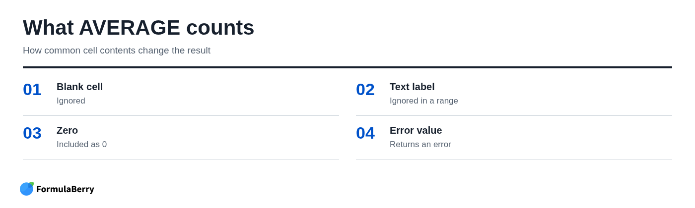
In a referenced range, Google Sheets generally ignores blank cells and text labels when calculating an average. Numeric zero, however, is a real value and is included in the calculation.

For example, if a range contains 80, 90, a blank, and 0, the average is 56.67 because Google Sheets averages three numeric values: 80, 90, and 0. It does not treat the blank as zero.

An error value such as #DIV/0!, #VALUE!, or #N/A is different. An error in the referenced data can cause the average formula to return an error as well. Handle source errors deliberately rather than assuming AVERAGE will skip them.

Average only cells that contain values

If your range has ordinary empty cells, you do not need a special formula. AVERAGE already ignores them.

The more difficult case is a cell that looks blank because it contains a formula returning an empty string, written as "". For example, a source formula might return a value only when an order is complete:

=IF(A2="Closed",C2,"")

When you need to make sure only nonempty displayed results are used, filter the range before averaging it:

=AVERAGE(FILTER(B2:B10,B2:B10<>""))

The FILTER portion keeps only cells in B2:B10 that are not empty strings, then AVERAGE calculates the result from the remaining values. For more ways to work with ranges that return multiple values, see Array Formula in Google Sheets: Examples and How to Use It.

When a blank-looking formula cell needs filtering

Suppose B2:B10 contains calculated commissions. Some rows have a formula that returns "" because the employee has not yet qualified for a commission. If you want an average only for rows showing a commission value, the FILTER approach makes that intent explicit.

Do not replace missing values with 0 unless zero is the real business value. A zero commission, zero sale, or zero score should lower the average; a missing or not-yet-calculated result often should not.

If the result still seems wrong, inspect one of the blank-looking cells in the formula bar. It may be truly empty, contain an empty string, or contain text that only resembles a number. Those cases can require different handling.

Use AVERAGEIF for one condition

Use AVERAGEIF when you want an average for records that meet one rule. Its structure is:

=AVERAGEIF(criteria_range, criterion, [average_range])

The criteria_range is where Google Sheets checks the condition. The criterion is the condition itself. The optional average_range contains the values to average when the condition is met. The same range-and-criterion pattern also appears in the COUNTIF formula in Google Sheets.

Average values for one category

Imagine column A contains sales regions and column C contains sales amounts. To calculate average sales for the East region, use:

=AVERAGEIF(A2:A100,"East",C2:C100)

Google Sheets checks A2:A100 for "East" and averages the corresponding cells in C2:C100.

If the same range should be tested and averaged, omit the final argument. For example, to average values in C2:C100 that are at least 80:

=AVERAGEIF(C2:C100,">=80")

Average values above or below a threshold

For numeric criteria written directly in a formula, put the comparison operator and number in quotation marks:

• =AVERAGEIF(C2:C100,">=80") averages values of 80 or higher.
• =AVERAGEIF(C2:C100,"<50") averages values below 50.
• =AVERAGEIF(C2:C100,">0") averages positive values only.

A common mistake is writing >=80 without quotation marks. Google Sheets needs it treated as a criterion, not as a standalone formula expression.

Use AVERAGEIFS for multiple conditions

Use AVERAGEIFS when a record must meet two or more conditions. The syntax is:

=AVERAGEIFS(average_range, criteria_range1, criterion1, ...)

This is useful when you need a more specific business answer, such as average revenue for one region and one order status, or average score for one course and one grading period.

Build a two-condition average

Assume column A contains regions, column B contains deal statuses, and column D contains revenue. To average revenue for closed deals in the East region, use:

=AVERAGEIFS(D2:D100,A2:A100,"East",B2:B100,"Closed")

The arguments are:

• D2:D100: the revenue values to average
• A2:A100: the range containing regions
• "East": the first condition
• B2:B100: the range containing statuses
• "Closed": the second condition

Every criteria range must line up with the average range. If D2:D100 is your average range, A2:A100 and B2:B100 must cover the same rows. Do not pair D2:D100 with A2:A50 or B3:B101; mismatched ranges can cause errors or misleading results.

Average visible rows in a filtered sheet

A regular AVERAGE formula includes hidden rows, which is often wrong for a filtered report. If you want the average to update when you filter the sheet, use:

=SUBTOTAL(1,C2:C100)

Function code 1 tells SUBTOTAL to calculate an average using visible rows in the range. For example, filter a sales report to show only one region, and the SUBTOTAL formula will recalculate based on the rows still visible.

This is not the same as averaging cells based on a value-based condition. Use AVERAGEIF or AVERAGEIFS when the condition belongs in the formula. Use SUBTOTAL when a person will control the visible records with a sheet filter.

There is one subtle distinction: SUBTOTAL(1,...) ignores rows hidden by a filter but includes manually hidden rows. If you also need manually hidden rows excluded, use function code 101:

=SUBTOTAL(101,C2:C100)

Avoid divide-by-zero and data errors in average formulas

If a Google Sheets average formula is not working, do not immediately wrap it in IFERROR. First identify whether the problem is an empty data set, a malformed criterion, mismatched ranges, or an error in the source cells.

When an empty result is the intended outcome, you can use:

=IFERROR(AVERAGE(B2:B10),"")

This displays a blank cell instead of an error. It is useful in dashboards and templates where data will be entered later. But IFERROR should not hide damaged source data that needs correction.

Why #DIV/0! appears

#DIV/0! usually means Google Sheets found no numeric values to average. That can happen when the range is empty, when numbers are stored as text, or when an AVERAGEIF or AVERAGEIFS formula finds no matching numeric records.

Check the relevant cells before changing the formula. A value that looks like 125 may be text because it was imported with an apostrophe, a currency symbol, or an inconsistent decimal format. Also check whether a filter or condition has left no qualifying rows.

Check ranges and criteria before changing the formula

Most broken conditional averages come down to one of these issues:

• Criteria ranges in AVERAGEIFS do not match the size of the average range.
• A text criterion is misspelled or contains an unexpected space.
• Numbers are stored as text in one column and as actual numeric values in another.
• The formula accidentally includes a header, subtotal, or grand total row.
• The selected range contains a source error such as #N/A.

Start by checking the range references in the formula bar. Then test the criterion on a small known set of rows before applying it to the entire sheet.

Choose the right average formula for your sheet

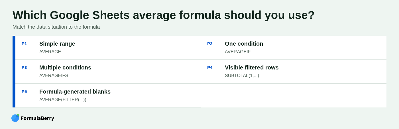
Use the formula that matches the question you are trying to answer:

Situation	Best formula
Average a normal numeric range	=AVERAGE(B2:B10)
Average values that meet one condition	=AVERAGEIF(A2:A100,"East",C2:C100)
Average values that meet multiple conditions	=AVERAGEIFS(D2:D100,A2:A100,"East",B2:B100,"Closed")
Average only visible rows after filtering	=SUBTOTAL(1,C2:C100)
Exclude formula-generated empty strings	=AVERAGE(FILTER(B2:B10,B2:B10<>""))

For percentages, use the same average formulas. The difference is formatting: format the result cell as a percentage rather than manually multiplying or dividing values unless your source data requires it. To show an average to two decimal places, format the result cell with two decimal places instead of altering the underlying calculation.

Apply these average formulas with confidence

Start with AVERAGE for a normal range of numbers. Move to AVERAGEIF when one condition matters, AVERAGEIFS when multiple conditions must be true, and SUBTOTAL when your active filters should determine the result.

Before trusting any average, confirm how your sheet treats zero values, blank-looking formula results, text-formatted numbers, and summary rows. Those details matter more than the formula name.

If you can describe the result you need but are unsure how to build the Google Sheets or Excel formula, FormulaBerry can generate, explain, or help correct the formula from a plain-language request.