A Google Sheets custom formula can look correct in the first row and quietly fail everywhere else. The usual culprit is not advanced math. It is a reference that moved when it should have stayed fixed, a blank cell that was never accounted for, or a conditional-formatting rule written for the wrong starting cell.

This guide covers both meanings of "custom formula" in Google Sheets: formulas you write for calculations and labels, and the custom formulas used to drive conditional formatting. You will learn how to write, copy, inspect, repair, and scale them without turning a working spreadsheet into a fragile one.

What a custom formula means in Google Sheets

People use "custom formula" in two related ways. First, it can mean any formula you create yourself, such as =B2*C2 for a line-item total or =IF(C2>500,"High value","Standard") for a label.

Second, and more commonly in discussions of formatting, it means a formula entered into a conditional-formatting rule. Instead of producing a value in a cell, that formula returns TRUE or FALSE. Google Sheets then applies formatting when the result is TRUE.

Both uses rely on the same fundamentals: clear logic, correct cell references, and deliberate handling of blanks and errors. The biggest difference is where the result goes: a normal formula displays an output, while a conditional-formatting formula controls an appearance.

Quick start: build a custom formula in five steps

Use this simple workflow whenever you need to make a custom equation in Google Sheets:

• Define the result. Decide exactly what the formula should return or identify.
• Choose the inputs. Identify the cells, columns, fixed settings, or lookup tables involved.
• Write the formula. Start with an equals sign and build the smallest useful version first.
• Test it in one blank cell. Confirm it works on a normal row and at least one edge case.
• Apply or copy it. Fill it down only after checking how references should move.

For example, if quantity is in B2 and unit price is in C2, enter =B2*C2 in D2 to calculate the line-item total. Test D2 first. Once it returns the expected amount, copy it down the column.

Formula anatomy: equals signs, functions, operators, and references

Every standard Google Sheets formula begins with an equals sign. After that, you can combine cell references, numbers, text, operators, and functions.

• Cell references point to data, such as A2 or $B$1.
• Operators perform an action or comparison. Examples include +, -, *, /, >, <, and <>, which means "not equal to."
• Functions are built-in instructions, such as SUM, IF, COUNTIF, and REGEXMATCH.
• Text values must be enclosed in quotation marks, as in "Overdue".

For instance, =SUM(B2:B10) adds a range of values. By contrast, =IF(C2>500,"High value","Standard") tests whether C2 is greater than 500 and returns one of two text labels. The IF function makes the decision; the > operator performs the comparison.

How to make a custom equation in Google Sheets

A reliable formula-building process works whether you are calculating totals, assigning labels, checking for missing information, or pulling a value from another table. Start in the first target cell, prove the logic there, and only then fill it through the dataset.

Do not begin by copying an unfinished formula down 500 rows. That makes debugging harder because you no longer know whether the problem is the logic, the source data, or the references.

Start with a plain-language rule

Before typing symbols, state the rule in ordinary language. For example: "Mark orders over $500 as high value. Leave empty order amounts blank."

That sentence contains everything you need:

• Input: the order amount in column C
• Condition: greater than 500
• Output: "High value" or "Standard"
• Blank behavior: do not label an empty row

A formula that follows the rule is =IF(C2="","",IF(C2>500,"High value","Standard")). Without the first test, blank rows would be labeled "Standard," which is technically consistent with the formula but usually wrong for the sheet.

Build and test the formula in a helper cell

Start with the smallest test. In a spare cell, enter =C2>500. Google Sheets returns TRUE when the order exceeds $500 and FALSE when it does not. That confirms the comparison works.

Next, turn the result into a label: =IF(C2>500,"High value","Standard"). Finally, add your blank-cell rule if needed: =IF(C2="","",IF(C2>500,"High value","Standard")).

Helper cells are especially valuable when you plan to use the same logic in conditional formatting. It is much easier to troubleshoot a visible TRUE or FALSE result in a cell than to guess why a row did or did not change color.

Cell references control what changes when you copy

Copying formulas safely depends on reference types. A reference tells Google Sheets where to look, but dollar signs tell it what is allowed to move when the formula is copied.

The practical rule is simple: lock the part of the reference that must not move.

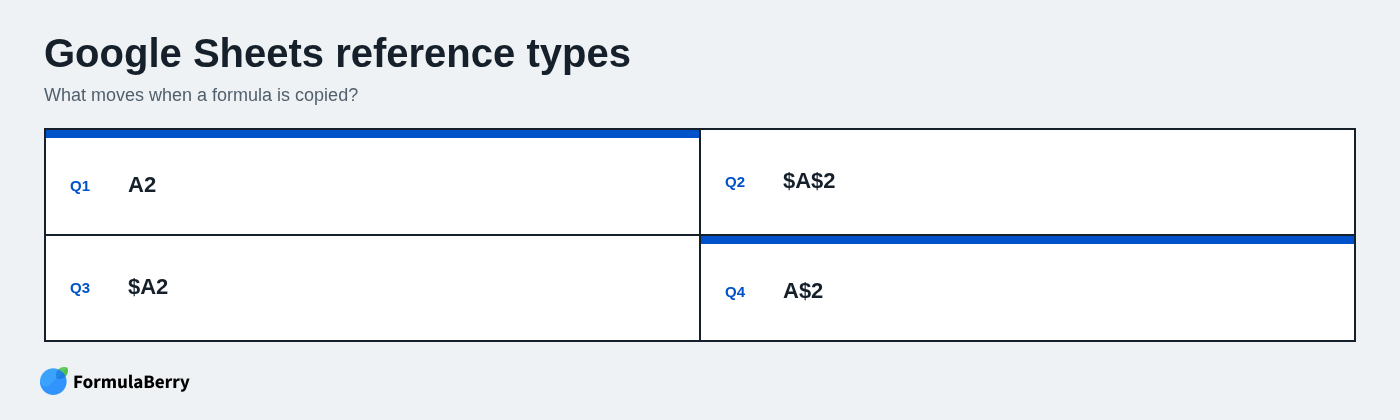
Relative references: A2

A relative reference changes both its row and column when copied. If D2 contains =B2*C2 and you copy it down one row, D3 becomes =B3*C3. Copy it one column to the right, and the references shift one column right as well.

This is exactly what you want for repeated row-level calculations, such as quantity multiplied by unit price for each order.

Absolute references: $A$2

An absolute reference locks both the column and row. If B1 contains a tax rate and you need every invoice line to use that one rate, use a formula such as =D2*$B$1.

When copied down, D2 changes to D3, D4, and so on, but $B$1 stays fixed. Absolute references are useful for thresholds, tax rates, exchange rates, configuration cells, and fixed lookup ranges.

Google Sheets provides ways to cycle through reference styles while editing a formula, but the essential skill is recognizing what should remain fixed before you copy.

Mixed references: $A2 and A$2

Mixed references lock only one part of the address. $A2 locks column A but lets the row change. A$2 locks row 2 but lets the column change.

They matter most in two-dimensional tables. Imagine a pricing grid with product names down column A and regions across row 1. A formula copied across and down may need to keep the product column fixed while allowing the current row to change, or keep the header row fixed while allowing the current column to change.

For example, if a scorecard formula needs the row label from A and the column target from row 1, a formula may use =$A2*B$1. The product or employee remains in column A, the factor remains in row 1, and the active data cell shifts normally.

Copy, fill, and paste formulas without breaking references

There are three different goals that people often call "copying a formula": copying a live formula that adapts to a new row, copying the displayed value only, and preserving the formula itself as visible text. Choose the method based on the goal.

Fill formulas down a column

For a continuous data table, write and verify the formula in the first target row. Then drag the fill handle down, copy and paste into the required range, or use the spreadsheet's fill behavior to extend through adjacent records where appropriate.

After filling, inspect the first, a middle, and the final populated row. If the formula should calculate =B2*C2 in row 2, it should be =B50*C50 in row 50, not a mixture of shifting and fixed references.

Be careful with blank gaps in your source data. Automatic fill behavior may stop at a gap, which can leave part of a column without formulas.

Keep references stable when copying

Dollar signs solve most unexpected changes. If every row should compare its amount in C against a threshold stored in H1, write =C2>$H$1. The C reference follows each row; H1 stays fixed.

Named ranges can make stable references easier to read. Instead of $H$1, you might name that cell HighValueThreshold and write =C2>HighValueThreshold. Use names consistently, particularly for settings and source tables that appear in multiple formulas. Naming every individual cell usually creates more maintenance work than it saves.

Paste formulas, values, or literal formula text intentionally

A normal paste copies the formula and adjusts relative references for the destination. That is useful when you want a live formula in a new location.

Paste values only when you need the current displayed results without the underlying formula. This is useful for exporting a final report, freezing a period-end total, or sharing a static snapshot.

If you need to document a formula rather than calculate it, store it as text. You can begin the entry with an apostrophe, such as '=IF(C2>500,"High value","Standard"), so Google Sheets displays the formula rather than evaluating it. This is useful in documentation tabs, formula dictionaries, and audit notes.

Show and explain formulas in Google Sheets

A formula is much easier to trust when you can see its structure and trace its inputs. That matters when you inherit a workbook, audit a report, or return to your own sheet six months later.

Use formula display for a sheet-wide audit

Selecting a formula cell lets you inspect its expression in the formula bar. For a larger audit, switch the sheet into formula-display mode so formulas appear in cells instead of calculated results.

This view is useful for spotting a row with a different reference pattern, an accidental hard-coded number, or a formula that stops early. Check your version of Google Sheets' Help menu for the current menu path or shortcut before documenting it for a team, as interfaces can change.

Formula display is not the same as storing a formula as text. Formula display temporarily reveals active formulas; text entries remain non-calculating documentation.

Use helper cells and named ranges to make logic readable

A long nested formula may be compact, but compact is not always maintainable. If you are calculating eligibility from an amount, a date, and a status, consider separating those checks into helper columns before combining the final result.

For example, one helper cell can test whether a date is overdue, another can test whether payment is unpaid, and a third can combine the two. The final logic is easier to audit than one deeply nested expression.

Named ranges help too. A formula like =IF(ActualSales>MonthlyTarget,"On track","Below target") is more readable than the equivalent collection of opaque addresses, provided the names are accurate and used consistently.

Custom formulas for conditional formatting: the core rules

Conditional formatting custom formulas are where reference mistakes become especially visible. They do not write a result into a cell. Instead, they evaluate each cell or row in the selected range and apply formatting when the formula returns TRUE.

Two rules matter most:

• The formula must evaluate to TRUE or FALSE.
• The formula is designed relative to the top-left cell of the range you selected.

Set up a custom formula rule

Start by selecting the range you want the rule to format. For example, select A2:F100 if you want formatting to affect full records from row 2 through row 100.

Then open conditional formatting, choose the custom-formula option, enter the test, choose the desired style, and verify the result with sample rows. Range selection comes first because it determines how the formula should be anchored.

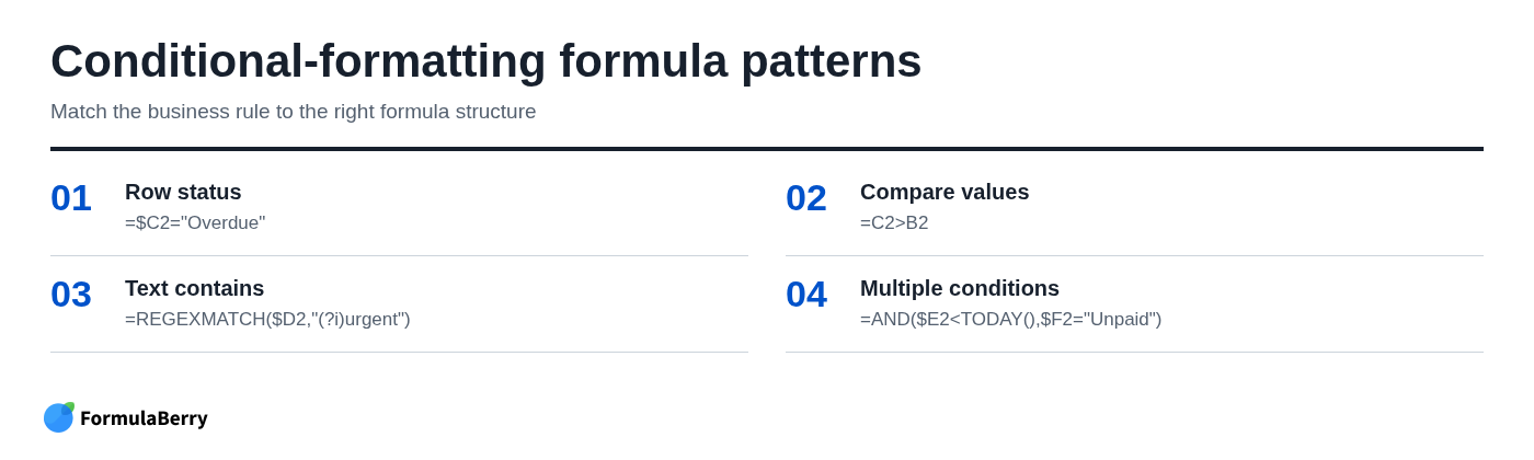
If your goal is to highlight every row whose status in column C is Overdue, use =$C2="Overdue" for the range A2:F100. The formula checks column C for each row, while the formatting applies across columns A through F.

Understand the top-left-cell rule

For the range A2:F100, Google Sheets evaluates the custom formula as though it begins at A2. It then adjusts relative references as it applies the rule through the range.

That is why =$C2="Overdue" works. The dollar sign keeps the check in column C even while formatting is applied to columns A through F. The row number is left relative, so row 2 checks C2, row 3 checks C3, and so forth.

A common mistake is writing =$C$2="Overdue". That locks the formula to C2 for every row, so the entire selected range may be formatted based solely on the status in the first row.

Google Sheets custom formula examples for conditional formatting

The patterns below cover the conditional-formatting rules most business spreadsheets actually need. In each case, the selected range is as important as the formula itself.

Highlight an entire row based on another cell

Apply to range: A2:F100
Formula: =$C2="Overdue"

This highlights every cell in a row when the value in column C is Overdue. The column is absolute because every cell in the formatted row must consult column C. The row stays relative because each record needs to evaluate its own status.

This pattern is the foundation for Google Sheets conditional formatting based on another cell. Replace "Overdue" with a dropdown value such as "Approved," "Blocked," or "Needs review" to match your workflow.

Format cells when one value is greater than another

Apply to range: C2:C100
Formula: =C2>B2

This highlights a value in column C when it exceeds the corresponding value in column B. For example, C may contain actual spending and B may contain the budget.

To highlight the full record instead, apply the rule to A2:F100 and use =$C2>$B2. Both columns are fixed so the whole row compares the correct two fields, while the row changes for each record.

Format text that contains a word or phrase

Apply to range: A2:F100
Formula: =REGEXMATCH($D2,"(?i)urgent")

This highlights rows where column D contains the word urgent, regardless of letter case. The (?i) part makes the match case-insensitive, so "URGENT," "Urgent," and "urgent" all match.

If you need a simpler contains check, you can use a SEARCH-based formula, but guard against blanks and errors. For example, =IF($D2<>"",ISNUMBER(SEARCH("urgent",$D2)),FALSE) returns FALSE for empty cells and avoids misleading results. Use REGEXMATCH when you need more flexible patterns; use a straightforward search when a plain word or phrase is enough.

Apply formatting when multiple conditions are true

Apply to range: A2:F100
Formula: =AND($E2<TODAY(),$F2="Unpaid")

This highlights a full row only when the due date in column E is before today and the payment status in column F is Unpaid. AND requires every condition to be true.

Use OR when any one condition should trigger the rule. For example, =OR($C2="Blocked",$C2="Escalated") can flag records needing attention under either status.

Use a custom formula with dates, blanks, and duplicates

Dates need special care because an empty cell can behave differently from a valid date, and text that looks like a date may not be recognized as one. A reliable overdue rule excludes blanks:

Apply to range: A2:F100
Formula: =AND($E2<>"",$E2<TODAY())

To flag missing required information, use a direct blank check:

Apply to range: A2:F100
Formula: =$B2=""

To find duplicates in a list of IDs in column A:

Apply to range: A2:A100
Formula: =AND(A2<>"",COUNTIF($A$2:$A$100,A2)>1)

The selected range defines the duplicate-checking scope. In this example, each ID is compared against A2:A100. The blank guard prevents empty cells from being highlighted simply because there are multiple blank rows. For more text-, number-, and date-based examples, see this guide to the COUNTIF formula in Google Sheets.

Worked example: build a deadline tracker with layered custom rules

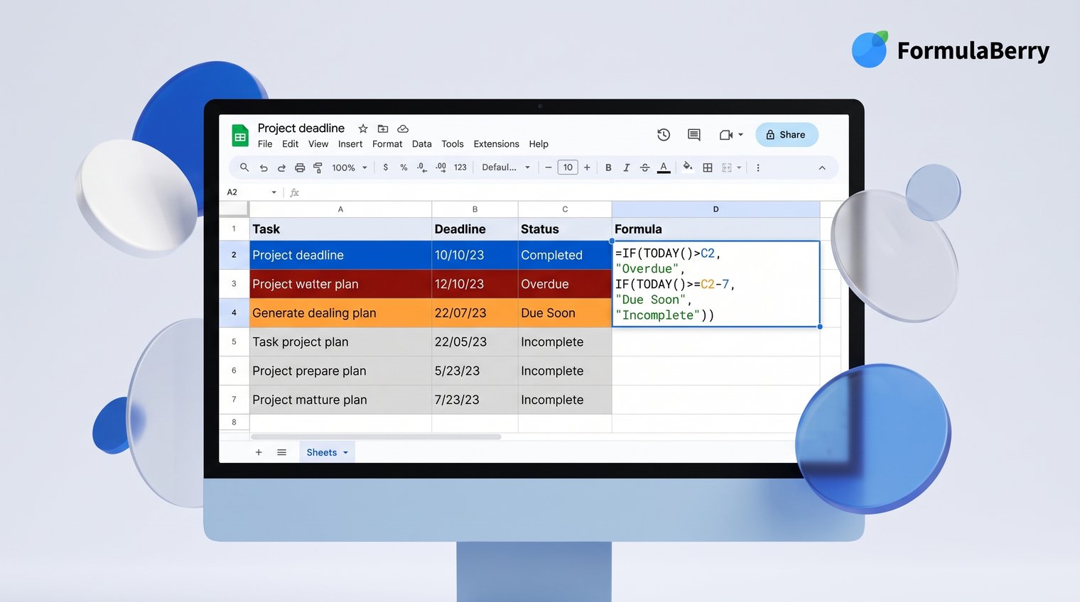
A deadline tracker is a good test of conditional formatting because several rules can apply to the same row. Assume the sheet has these columns: A for Task, B for Owner, C for Due Date, D for Status, and E for Priority.

Define the formatting logic before writing formulas

Set the visual hierarchy before opening the formatting panel:

• Completed rows should be muted.
• Incomplete overdue rows should be red.
• Tasks due soon should be amber.
• Rows with no owner should be flagged.

Precedence matters. A completed task with an old due date should look completed, not overdue. Decide that rule now rather than discovering conflicting colors after the sheet is in use.

Write each rule with the right anchors

Apply all of the following rules to A2:E200 so each one can format an entire task row.

Completed, muted:
=$D2="Completed"

Overdue and not completed, red:
=AND($C2<>"",$C2<TODAY(),$D2<>"Completed")

Due within the next three days and not completed, amber:
=AND($C2>=TODAY(),$C2<=TODAY()+3,$D2<>"Completed")

Missing owner, flagged:
=AND($A2<>"",$B2="",$D2<>"Completed")

In each rule, the column letters are locked because the formula must always check the same fields: due date in C, status in D, and owner in B. The row remains relative so the rule evaluates the corresponding cells for each task.

Test edge cases and adjust rule order

Create a few deliberate test rows before relying on the tracker:

• A completed task with a date last month
• An incomplete task due yesterday
• An incomplete task due tomorrow
• A new task with no due date
• A task with a date stored as text instead of a real date
• A task with no owner

If a completed overdue task still appears red, check whether the overdue formula excludes completed status and whether the completed rule is ordered to take priority. If blank due dates are flagged as overdue, add the $C2<>"" condition. If dates stored as text do not behave as expected, correct the underlying data rather than adding increasingly complicated workarounds to every rule.

Build more reliable custom formulas with functions and error handling

Reliable formulas do not merely produce the right result for ideal data. They make a deliberate choice about missing values, bad inputs, and conditions that change as the sheet grows.

Use IF, IFS, AND, OR, and NOT for decision logic

Use IF when there are two clear outcomes. For example, =IF(D2="Paid","Closed","Open") is easy to read and sufficient for a binary status.

Use IFS when several ordered outcomes are more readable than nested IF statements. For example, a priority label might use conditions for overdue, due soon, and future work. Use AND when all conditions matter, OR when any condition is enough, and NOT when you need to exclude a state.

Do not force elaborate logic into one formula just because it is possible. As covered in the helper-cell section, intermediate checks often make a sheet safer to maintain.

Handle blanks and errors deliberately

ISBLANK, LEN, and direct comparisons to an empty string can help identify missing values. In many worksheets, =A2="" is a practical blank check because it also catches cells whose formula returns an empty string.

Use IFERROR carefully. It is useful when a missing lookup should produce a friendly fallback, such as =IFERROR(XLOOKUP(A2,ProductIDs,ProductNames),"Unknown product"). But do not use IFERROR to hide every issue. A formula error can reveal bad source data, a broken range, or an unexpected change that needs attention.

For calculations, guard against empty inputs before calculating. A formula such as =IF(OR(B2="",C2=""),"",B2*C2) prevents a blank line from displaying an unhelpful zero or error.

Use lookup and array formulas only when they reduce repetition

Lookups are useful when a sheet needs to retrieve matching information from a reference table. XLOOKUP, where available in your Sheets environment, or an INDEX/MATCH pattern can retrieve a price, category, owner, or target based on an ID.

Array formulas can apply one expression to a larger range automatically, reducing repeated row-by-row formulas. They also require room to expand. If cells below the formula already contain content, the array cannot spill its results correctly. For practical patterns, see this guide to array formulas in Google Sheets.

Use these tools when they clearly reduce repetitive maintenance. For a small, readable sheet, a conventional formula filled down can be easier for the next person to understand.

How to fix a Google Sheets formula that is not working

Random edits are a slow way to debug. Instead, start with the smallest possible test, verify data and references, then rebuild complexity one piece at a time.

Check syntax, separators, and data types first

Look for missing parentheses, unmatched quotation marks, misspelled function names, and misplaced commas. In some spreadsheet locales, formulas use semicolons instead of commas as argument separators, so a correct-looking formula copied from another source may fail immediately.

Then inspect the underlying data. A number stored as text may not compare or calculate as expected. A date that looks valid may actually be plain text. Test a suspect input in a separate cell rather than assuming its format tells the whole story.

If a formula is long, isolate components. Test the comparison first, then the function input, then each condition. Find the first step that produces an unexpected result.

Check references and range sizes

A #REF!-style problem often means a referenced cell, column, or sheet was deleted or moved. In array formulas, mismatched range dimensions can also cause failures. Verify that related ranges start and end on compatible rows.

For copied formulas, confirm that absolute and mixed references are locked correctly. A missing dollar sign can make a lookup table slide down one row at a time, producing results that appear plausible but are wrong.

For conditional formatting, revisit both the selected range and the top-left reference. A correct formula written for A2:F100 may fail when applied to A1:F100 because every row reference is now offset by one.

Debug a formula by simplifying it

Use a repeatable sequence:

• Test the most basic comparison, such as =C2>500.
• Test each function input independently.
• Add one condition at a time with AND, OR, or IF.
• Confirm behavior on a known-good row.
• Test a blank, an error-prone input, and an unusual but valid case.
• Add error handling last, after the base logic works.

This method prevents an error wrapper from hiding the actual defect. It also works for conditional formatting: test the formula in a helper cell first, confirm that it returns TRUE for the intended row, then place it in the rule.

Use an AI formula generator without losing control of the logic

Natural-language formula assistance is useful when you know the business rule but cannot immediately translate it into spreadsheet syntax. It can also help explain inherited formulas and suggest corrections to a formula that is close but not working. If you want more guidance on this workflow, see the Google Sheets Formula Generator guide.

It should not replace verification. A generated formula can still use the wrong columns, make a poor assumption about blanks, or lock references incorrectly for your target range.

Write prompts that produce usable Google Sheets formulas

A vague request such as "highlight overdue invoices" leaves too much open. A useful request identifies the columns, rule, blank behavior, target range, and whether the formula is for a cell or conditional formatting.

For example:

In Google Sheets, create a conditional-formatting formula for A2:F200. Highlight the full row when the due date in column E is before today and the payment status in column F is Unpaid. Ignore blank due dates. Keep columns E and F fixed while the row changes.

That prompt gives the assistant enough detail to produce the intended pattern: =AND($E2<>"",$E2<TODAY(),$F2="Unpaid").

Review generated formulas before filling a sheet

Before copying any generated formula through a workbook, check five things:

• Does the output match the stated business rule?
• Are relative, absolute, and mixed references appropriate?
• Does the formula handle blanks as intended?
• Is the range scope correct for lookups, duplicates, arrays, or formatting?
• Does it work on a normal sample row and an edge case?

For a conditional-formatting request, review the apply-to range and formula together. A perfect formula attached to the wrong range is still the wrong rule.

FormulaBerry

The screenshot shows FormulaBerry's plain-language request workflow, where you describe a Google Sheets task before generating or explaining a formula. FormulaBerry is designed for people who need help generating, explaining, or correcting formulas for Google Sheets and Microsoft Excel from a plain-language request.

For example, you can describe the columns involved, explain how blanks should behave, and ask for a conditional-formatting formula or a regular cell formula. You can also use it to unpack a complex formula you inherited before changing it.

The important limitation is that FormulaBerry is a formula assistant, not a replacement for your spreadsheet or a fully automated data-analysis system. You still need to confirm the column layout, selected range, data types, and expected results in your own sheet. That makes it a strong fit for spreadsheet users who want faster formula drafting and clearer explanations without giving up control of the logic.

A practical checklist for every Google Sheets custom formula

Use this checklist before filling a formula down a column or relying on a conditional-formatting rule:

• Desired result: Can you state the rule in one plain-language sentence?
• First-row test: Does it work correctly in the first intended cell or row?
• References: Have you locked the rows and columns that must remain fixed?
• Blanks: What should happen when an input cell is empty?
• Errors: Are errors useful signals, or is a controlled fallback appropriate?
• Range scope: Does the lookup, duplicate check, array output, or formatting rule cover the right area?
• Edge cases: Have you tested unusual but valid data, including text-formatted numbers or dates?
• Conditional formatting: Is the formula written relative to the top-left cell of the apply-to range?

Create custom formulas that stay accurate as your sheet grows

The best Google Sheets custom formulas are not necessarily the shortest. They are the ones with a clear rule, intentional references, sensible blank behavior, and enough testing to survive new rows and changing data.

Start with plain language, test the first row before copying, and use dollar signs only where they serve a purpose. For conditional formatting, always design the formula around the top-left cell of the selected range and test competing rules together.

When a formula is difficult to write, explain, or repair, FormulaBerry can help turn your requirement into a starting formula. Review the output against real sample data, then keep the logic documented so the sheet remains reliable long after it leaves your hands.