

To pull data from one Google Sheets file into another, use the Google Sheets IMPORTRANGE formula. It imports a selected range from a separate spreadsheet and updates when the source changes. If the data is on another tab in the same spreadsheet, however, IMPORTRANGE is the wrong tool - use a direct tab reference instead.
The formula itself is simple. Most problems come from permissions, an incorrect tab name, or trying to place an expanding import on top of existing data.
What IMPORTRANGE does and when to use it
IMPORTRANGE pulls a specified cell range from one Google Sheets spreadsheet file into another. For example, a manager could keep raw order data in one file and bring selected order columns into a separate reporting workbook.
Use it when the source and destination are different Google Sheets files. The first time you connect two files, Google Sheets asks you to approve the connection by selecting Allow access. After that, changes in the source can flow through to the destination automatically, though updates are not always instantaneous.
Do not use IMPORTRANGE just to reference another tab in the same workbook. A direct reference is cleaner and faster:
='Sales Data'!A1:D20
IMPORTRANGE formula syntax
The syntax is:
=IMPORTRANGE(spreadsheet_url, range_string)
spreadsheet_url is the URL of the source Google Sheet. range_string identifies the source tab and the cells to import using A1 notation. Put the range string in quotation marks, including the tab name and exclamation point.
Here is a basic example:
=IMPORTRANGE("https://docs.google.com/spreadsheets/d/FILE_ID/edit", "Orders!A2:F")
This imports columns A through F from row 2 onward on the Orders tab. Replace the URL and tab name with your own details.
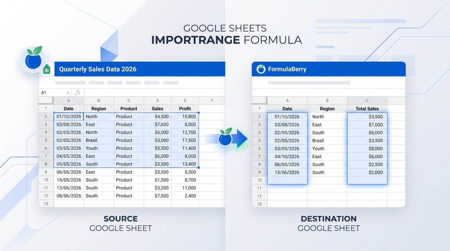
How to import data from one Google Sheet to another
To create an import, open the destination spreadsheet first. Click the cell where the imported data should begin, enter your IMPORTRANGE formula, and press Enter.
- Copy the URL of the source spreadsheet.
- Enter an IMPORTRANGE formula in the destination file.
- Press Enter.
- When prompted, select Allow access.
- Confirm that the imported rows and columns appear as expected.
Start small. Rather than immediately importing thousands of rows, test a known range such as "Orders!A1:F10". That makes it easier to catch a misspelled tab name, the wrong columns, or an unwanted header row before you build formulas and charts around the data.
Remember that IMPORTRANGE returns an expanding array. The destination cells below and to the right of the formula must be empty, or the import cannot expand. For more on formulas that return multiple results, see this guide to Array Formula in Google Sheets.
Examples for common IMPORTRANGE tasks
Each example below uses source_url as a placeholder. Replace it with the full URL of the source spreadsheet, then adjust the tab name and range for your own workbook.
Import a fixed table range
Use a bounded range when the imported table has a known size or when you want a stable dashboard input.
=IMPORTRANGE("source_url", "Inventory!A1:G50")
This imports rows 1 through 50 and columns A through G from the Inventory tab. It is a sensible choice for a curated table, a monthly report, or a dashboard that should not pull in blank rows far below the active data.
Import entire columns that grow over time
For a lead list, transaction log, or other table that receives new rows, import open-ended columns:
=IMPORTRANGE("source_url", "Leads!A:K")
This approach picks up rows added later without changing the formula. The trade-off is performance: importing many full columns from a very large spreadsheet can slow a workbook down. Import only the columns you actually need.
Import a single cell or a small summary block
IMPORTRANGE is also useful for KPI rollups. A leadership dashboard may need one revenue figure from each team file rather than every underlying transaction. If you need to calculate totals in the destination, see this guide to the Google Sheets SUM formula.
=IMPORTRANGE("source_url", "Dashboard!B4")
To bring in a compact summary table instead, use:
=IMPORTRANGE("source_url", "Dashboard!B4:D8")
How to pull data from another tab in the same spreadsheet
For another tab in the same spreadsheet file, use a standard sheet reference. It updates automatically and does not require an Allow access step.
If the tab name contains no spaces:
=Sheet2!A1:D20
If the tab name contains spaces, wrap it in apostrophes:
='Q1 Sales'!A1:D20
This distinction matters. Direct references are the better choice for same-file reporting because they avoid a separate cross-file connection and keep formulas simpler.
Filter, query, and sort imported data
IMPORTRANGE moves the data; functions such as FILTER, QUERY, and SORT shape it in the destination spreadsheet. First make sure the base import works and has been authorized, then add the wrapper formula.
Import only matching rows with FILTER
To pull only orders marked Open, use FILTER around imported ranges:
=FILTER(IMPORTRANGE("source_url","Orders!A2:F"), IMPORTRANGE("source_url","Orders!C2:C")="Open")
This works, but it calls IMPORTRANGE twice. In a more complex workbook, that can create unnecessary overhead. A better structure is often to import raw data once into a dedicated helper tab, then run FILTER against the local imported range.
Select and filter columns with QUERY
Google Sheets QUERY is often more compact when you need to choose columns and filter rows at the same time:
=QUERY(IMPORTRANGE("source_url","Orders!A1:F"), "select Col1, Col3, Col6 where Col4 = 'Open'", 1)
Within QUERY, imported columns are referenced as Col1, Col2, and so on, based on their position in the imported range. The final 1 tells Google Sheets that the first imported row is a header row.
Sort an imported range
To sort leads by the fourth column of the imported range in descending order:
=SORT(IMPORTRANGE("source_url","Leads!A2:D"), 4, FALSE)
The 4 means the fourth column within the imported result. It does not refer to the original column letter in every possible source range. If you imported C:F, for example, position 4 would correspond to source column F.

Fix common IMPORTRANGE errors
Most IMPORTRANGE errors have a straightforward cause. Check access and the source reference before rebuilding the formula from scratch.
#REF! error and the Allow access button
A #REF! error commonly appears when the destination file has not been approved to access the source file. Click the cell containing the formula and select Allow access.
If the button does not resolve the issue, verify that the Google account you are using can open the source spreadsheet. You cannot import data that your account has not been permitted to view.
Range not found or a formula parse error
Check the source tab name carefully. The range string needs quotation marks, an exclamation point between the tab name and cell range, and valid A1 notation.
For tabs with spaces, the apostrophes belong inside the quoted range string:
=IMPORTRANGE("source_url", "'January Orders'!A1:F")
To isolate the problem, try a small known-valid reference such as "Sheet1!A1". If that works, the issue is likely in the larger range rather than the spreadsheet URL.
Imported data will overwrite existing data
This message means the formula has no clear space to expand. IMPORTRANGE can return multiple rows and columns, so any content in its expected spill area blocks the result.
Clear or move the conflicting cells, reduce the imported range, or place the formula on a dedicated import tab. Keeping raw imports away from manually entered content prevents this problem from returning later.
Loading, slow refreshes, or too much data
Large, repeated imports can make a spreadsheet feel sluggish. Reduce the range to required columns and rows, avoid chains of IMPORTRANGE formulas across several files, and keep one raw import as the source for downstream calculations.
Google Sheets updates imported data automatically, but it should not be treated as an instant data pipeline. For operational reporting, design the workbook so a short delay does not cause decisions or formulas to fail.
Build a more reliable IMPORTRANGE workflow
The most reliable setup separates data transfer from analysis. Keep stable headers in the source sheet, create one designated raw-import area in the destination workbook, and build calculations, pivot-style summaries, and charts on separate tabs.
This layout makes troubleshooting much easier. If a report looks wrong, you can first inspect the raw import to determine whether the issue began in the source file, the import range, or a downstream formula.
Access management also matters in shared workbooks. People viewing the destination sheet may need appropriate access to the source file, and permission or ownership changes can interrupt an established connection. For recurring operational spreadsheets, document the source URL, source tab, and file owner somewhere the team can find them.
Use the right reference and keep imports maintainable
Use a direct tab reference when the data lives in the same spreadsheet, and use IMPORTRANGE when it lives in another file. Get the basic import working first, then add QUERY, FILTER, or SORT only when the destination needs a shaped reporting view.
A small, clearly defined import range is usually more maintainable than a workbook full of broad, repeated formulas. When you need help generating, explaining, or correcting a Google Sheets formula, FormulaBerry can turn the result you want into a formula you can use.