

QUERY is one of the most useful Google Sheets functions and one of the easiest to break. A missing quote, the wrong column reference, or a date in the wrong format can turn a clean report into a parse error or an empty result.
Once you understand its structure, though, QUERY can replace a surprising amount of manual filtering, sorting, copying, and summarizing. This guide covers the syntax, the clauses that matter, practical report examples, and the fixes for the problems that trip up most spreadsheet users.
What the Google Sheets QUERY Function Does - and When to Use It
The Google Sheets QUERY function turns a table of data into a formula-driven report. It can select columns, filter rows, sort results, group records, calculate totals, and create pivot-style summaries using one formula.
Use QUERY when you need a repeatable output that updates as source data changes. For example, you might have a sales log with hundreds of rows but need a separate table showing only East region orders over $500, sorted from largest to smallest.
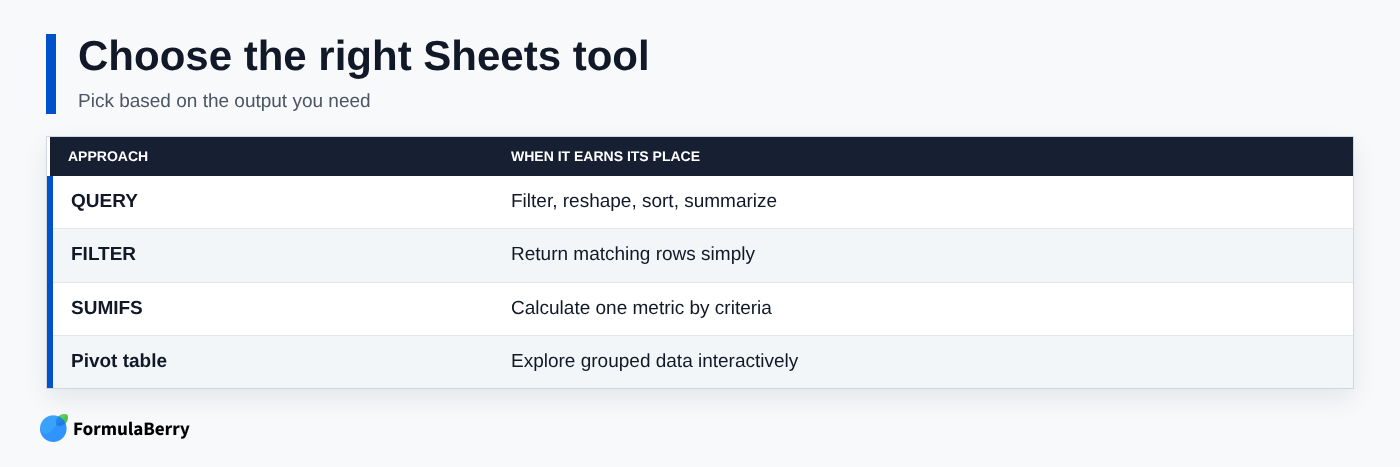
It is not always the best tool. FILTER is often simpler when you only need matching rows. SORT is better for straightforward ordering. SUMIFS is excellent when you need one number, such as monthly revenue for a region. Pivot tables are often easier when people need to explore data interactively.
QUERY is the stronger choice when several steps need to happen together: filter, rearrange columns, sort, and summarize in a single reusable report.
Quick start: the smallest useful QUERY formula
Here is a basic formula:
=QUERY(A1:D10,"select A, B, D",1)
This tells Google Sheets to look at the range A1:D10 and return columns A, B, and D. The 1 at the end means the range contains one header row.
The general pattern is simple: provide data, write instructions in a query string, then state how many header rows appear in the source range.

QUERY Formula Syntax: Range, Query String, and Headers
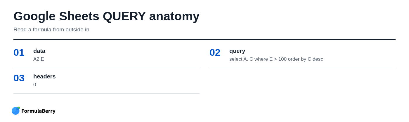
Every QUERY formula follows this structure:
=QUERY(data, query, [headers])
data is the range or array you want to analyze. query is the text instruction that tells Sheets what to return. headers is optional, but specifying it deliberately avoids many confusing results.
For a simple report, the formula might look like this:
=QUERY(A1:E,"select A, C, E where E > 100",1)
The query text is inside double quotation marks. If you need to insert a value from another cell, you build the query string with concatenation instead of writing the entire instruction as one fixed piece of text.
The data range and column identifiers
When QUERY reads a direct spreadsheet range, such as A1:E or Sales!A:E, refer to columns by letter: A, B, C, and so on.
When QUERY reads an array created with curly braces or output from functions such as IMPORTRANGE, use numbered identifiers instead: Col1, Col2, Col3. If you need to review how array-based outputs work more broadly, see this guide to Array Formula in Google Sheets: Examples and How to Use It.
For example, this direct-range formula uses letters:
=QUERY(A1:D,"select A, D where B = 'East'",1)
This array formula uses numbered columns:
=QUERY({Jan!A2:D;Feb!A2:D},"select Col1, Col4 where Col2 = 'East'",0)
Do not mix the two identifier styles. A direct range expects A, B, and C. An array-based source expects Col1, Col2, and Col3.
The query language clauses you will use most
You do not need to memorize the entire QUERY language. Most useful formulas are built from a small group of clauses:
- select chooses columns or calculations to return.
- where filters records by a condition.
- order by sorts the result.
- limit returns only a set number of rows.
- offset skips rows before returning results.
- label changes output headers.
- group by groups records for summaries.
- pivot turns category values into columns.
- format controls how certain output values display.
Think of the clauses as instructions written in sequence. First choose what to return, then filter it, then group or sort it as needed.
Prepare Your Source Data Before You Query It
Most QUERY problems begin in the source table, not in the formula. QUERY works best with a rectangular range: one row of consistent headers followed by records arranged in predictable columns.
Keep one data type in each column where possible. A Revenue column should contain numbers, not a mix of numbers, currency text, and entries such as "TBD." A Date column should contain real spreadsheet dates, not a mixture of dates and typed text.
Avoid merged cells inside source data. Merged cells may look tidy in a human-facing report, but they create unreliable structures for formulas. Keep the raw table plain and use a separate report tab for presentation.
Choose the correct header count
The last QUERY argument tells Sheets how many header rows are in the selected range. In practice, the most common values are 1 and 0.
Use 1 when your range begins with a single header row:
=QUERY(A1:D,"select A, B, D",1)
Use 0 when the range starts with data:
=QUERY(A2:D,"select A, B, D",0)
If you use the wrong count, Sheets may treat your first record as a header and omit it from the results. It may also produce generic output labels such as Col1 rather than using your actual field names.
Resolve mixed-type columns before writing the query
QUERY determines the dominant data type in a column. Values that do not match the majority type can be treated as null, which is why a seemingly valid filter can exclude records you expected to see.
For example, if most values in column D are numbers but several cells contain text such as "n/a," those text values may not behave as ordinary records in a numeric query.
Clean the source data before building the report. Use helper columns if necessary: convert numeric-looking text with VALUE, standardize dates with DATEVALUE, and remove excess spaces with TRIM. A helper column is often more maintainable than forcing a complicated cleanup operation into an already long QUERY formula.
Select Specific Columns and Rename the Output
A common reason to use QUERY is to create a focused report from a much wider source table. Rather than copying data into a second sheet and manually hiding columns, select only the fields people need to see.
Select columns in a different order
Suppose columns A through E contain Order ID, Date, Customer, Region, and Revenue. To create a report showing Customer first, then Order ID, then Revenue, use:
=QUERY(A1:E,"select C, A, E",1)
The source table remains unchanged. QUERY simply creates a different view of it, which is safer than rearranging columns in data that other formulas may depend on.
Use LABEL to create reader-friendly column names
QUERY can rename output columns with the label clause. This is preferable to manually typing over a QUERY result, because formula outputs can expand or refresh.
For a grouped revenue report, use:
=QUERY(A1:E,"select C, sum(E) where C is not null group by C label C 'Customer', sum(E) 'Revenue'",1)
If a label itself needs an apostrophe, double it inside the query text. For example, 'Customer''s Revenue' produces the label Customer's Revenue.
Filter Rows with WHERE Conditions
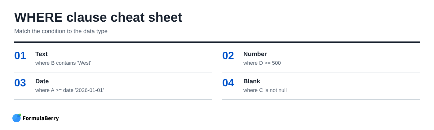
The where clause is the core of most QUERY formulas. It lets you create a query with condition logic for text, numbers, dates, and blank cells.
Text values are placed in single quotes inside the query string. Numbers are generally written without quotes. That distinction matters.
For example:
=QUERY(A1:E,"select A, C, E where D = 'East'",1)
Here, D is compared with the text value East. A numeric condition looks different:
=QUERY(A1:E,"select A, C, E where E > 500",1)
Match text with equals, contains, starts with, and matches
Use an equals sign when the cell must match exactly:
where B = 'East'
Use contains when the value can appear anywhere in the text:
where C contains 'trial'
Use starts with or ends with when the position matters:
where C starts with 'New'
where C ends with 'Ltd'
The matches operator uses regular expressions, or regex. Regex is a pattern-matching syntax that is useful when one condition needs to match several variations. For example:
where B matches 'East|West'
This returns rows where column B is exactly East or West. Use matches carefully: it is more powerful than contains, but it is less forgiving when the pattern is written incorrectly.
Filter numeric values and date ranges
For numeric data, use ordinary comparison operators:
where D >= 500
where D < 1000
To create a range, combine two conditions:
where D >= 500 and D <= 1000
Dates require special syntax. QUERY expects a date literal written as date 'yyyy-mm-dd', regardless of how the date displays in your spreadsheet. For related month-end calculations, see this guide to the Google Sheets end of month formula.
=QUERY(A1:E,"select A, B, E where A >= date '2026-01-01' and A <= date '2026-03-31'",1)
Do not write dates as 1/1/2026 or 01-01-2026 in the query text. Those display formats may be valid in a cell, but they are not valid QUERY date literals.
Find blanks, non-blanks, and combine conditions
Use is null to find blank values and is not null to keep filled values:
where C is null
where C is not null
Combine conditions with and or or. Parentheses make multi-condition logic easier to read and less likely to return the wrong rows.
For example, this Google Sheets query with multiple conditions returns East or West region orders with at least $500 in revenue:
=QUERY(A1:E,"select A, B, C, E where (D = 'East' or D = 'West') and E >= 500",1)
Build and test conditions one at a time before combining them. That is the fastest way to identify whether the issue is the region value, the revenue data type, or the logic itself.
Sort, Limit, and Paginate Results with ORDER BY
Filtering is usually more useful when the returned records are in a sensible order. The order by clause sorts QUERY results without changing the original source table.
Place it after select and where clauses. For example:
=QUERY(A1:E,"select A, C, E where E > 0 order by E desc",1)
This returns positive-revenue rows and sorts them from highest to lowest revenue.
Sort by one or more columns
Use asc for ascending order and desc for descending order:
order by D desc
To sort by more than one field, separate the fields with commas:
order by B asc, D desc
That pattern might sort a report alphabetically by customer, then place each customer's largest orders first. In straightforward direct-range queries, Sheets can often sort by a column even if you do not return it. Still, including key report fields usually makes the formula easier for another person to understand and maintain.
Return a top-N list with LIMIT and OFFSET
Use limit to return only a specified number of rows. A top-five sales report might use:
=QUERY(A1:E,"select A, C, E where E is not null order by E desc limit 5",1)
offset skips results. If the top five are already displayed elsewhere, this returns the next five:
=QUERY(A1:E,"select A, C, E where E is not null order by E desc limit 5 offset 5",1)
This can support simple paginated views, although most operational spreadsheets are clearer when they use filters or separate report sections rather than forcing users to move through pages of rows.
Summarize Data with GROUP BY, Aggregates, and PIVOT
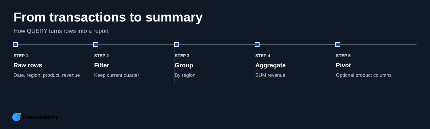
QUERY becomes much more powerful when it summarizes transactions rather than merely listing them. Aggregates such as sum, avg, count, min, and max let you turn a raw data table into a management report.
The key rule is simple: every selected field that is not aggregated must also appear in the group by clause.
Build a grouped summary table
Assume column B contains regions and column D contains revenue. This formula totals revenue by region:
=QUERY(A1:D,"select B, sum(D) where B is not null group by B label sum(D) 'Total'",1)
Column B is not aggregated, so it appears in group by B. Column D is aggregated through sum(D).
You can extend the same idea. For example, a report could group by Region and Product, calculate total revenue, and sort the grouped results from largest to smallest. As covered in the section on filtering, add a where clause before the group by clause when you want the summary to include only a particular period or status.
For example:
=QUERY(A1:E,"select D, sum(E) where A >= date '2026-01-01' group by D order by sum(E) desc label D 'Region', sum(E) 'Revenue'",1)
Create a formula-driven pivot report
The pivot clause creates columns from category values. It is useful for repeatable reports that should update automatically without someone rebuilding a pivot table.
For example, if column B is Region, column C is Product, and column D is Revenue:
=QUERY(A1:D,"select B, sum(D) where B is not null group by B pivot C label sum(D) 'Revenue'",1)
The result shows one row per region and separate revenue columns for each product. Keep enough empty columns to the right of the formula, because pivot output expands horizontally when new category values appear.
A standard pivot table may still be better for ad hoc analysis. Choose QUERY when the report must live in a fixed location, update automatically, and follow a consistent formula-based structure.
Use QUERY with Another Sheet, Multiple Sheets, and IMPORTRANGE
QUERY can use data from another tab, combine matching data from multiple tabs, or analyze a range imported from a different Google Sheets file. The important requirement is a consistent schema: matching columns in the same order with compatible data types.
Query data from another tab in the same spreadsheet
For a tab name with spaces, wrap the name in single quotes:
=QUERY('January Sales'!A1:E,"select A, C where E > 0",1)
This is the simplest form of a Google Sheet QUERY from another sheet. The formula can sit in any tab in the same workbook while the data stays in its original location.
Query multiple sheets with stacked arrays
To combine monthly tabs with identical layouts, stack them vertically using curly braces and semicolons:
=QUERY({Jan!A2:D;Feb!A2:D;Mar!A2:D},"select Col1, Col2, sum(Col4) group by Col1, Col2",0)
Because the source is now an array literal, use Col1, Col2, and so on rather than A, B, and C.
Each appended range must have the same number of columns in the same order. If January has Date, Region, Product, Revenue but February has Date, Product, Region, Revenue, the combined report will be wrong even if the formula does not show an error.
Use IMPORTRANGE as the QUERY data source
To query a separate spreadsheet, nest IMPORTRANGE inside QUERY:
=QUERY(IMPORTRANGE("spreadsheet_url","Data!A:E"),"select Col1, Col3 where Col5 > 100",1)
The first time you connect two spreadsheets, Google Sheets asks you to allow access. After that one-time connection, the formula can refresh from the source workbook.
Use Col identifiers with IMPORTRANGE output. Also remember that imported data inherits its source quality problems: inconsistent dates, text numbers, and unexpected blanks still need to be cleaned before you rely on a report.
Make QUERY Criteria Dynamic with Cell References
Hard-coded criteria are fine for a one-off analysis. For a report others will use, it is usually better to place selections in input cells and build the query around them.
For instance, a user could choose a region in H2, a minimum revenue threshold in H3, and a date range in H4:H5. The output updates without anyone editing the formula itself.
Insert text and numeric criteria from cells
To use text from a cell, concatenate it into the query string and place single quotes around the inserted value:
=QUERY(A1:E,"select A, C, E where D = '"&H2&"'",1)
If H2 contains East, the final query behaves like where D = 'East'.
For a numeric threshold, do not add single quotes:
=QUERY(A1:E,"select A, C, E where E >= "&H3,1)
Use data validation for input cells where possible. A dropdown for region names reduces misspellings and prevents a user from entering a value that does not exist in the source table. For unrestricted text input, escape apostrophes before concatenating the value: SUBSTITUTE(H2,"'","''").
Build date criteria from cells with TEXT
Date input cells need extra formatting because QUERY requires yyyy-mm-dd date literals. If F1 contains a valid start date, use:
=QUERY(A1:E,"select A, C, E where A >= date '"&TEXT(F1,"yyyy-mm-dd")&"'",1)
For a date range using F1 as the start date and G1 as the end date:
=QUERY(A1:E,"select A, C, E where A >= date '"&TEXT(F1,"yyyy-mm-dd")&"' and A <= date '"&TEXT(G1,"yyyy-mm-dd")&"'",1)
The source cell can display January 1, 2026, 1/1/2026, or another local format. The TEXT function converts it into the exact literal QUERY needs.
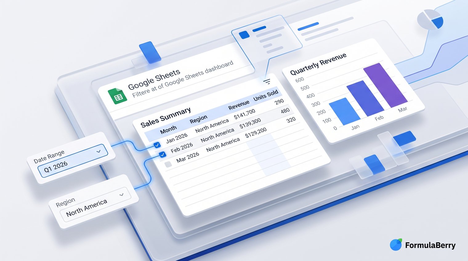
A Worked Example: Build a Dynamic Sales Dashboard Table
Suppose a Sales tab contains this structure:
- Column A: Order Date
- Column B: Order ID
- Column C: Customer
- Column D: Region
- Column E: Product
- Column F: Revenue
On a Dashboard tab, create four controls:
- H2: Region
- H3: Start Date
- H4: End Date
- H5: Minimum Revenue
Use a dropdown in H2 with values such as All, East, West, North, and South. Keep H3 and H4 as real date cells, not typed date text.
Start with a plain selected view:
=QUERY(Sales!A1:F,"select A, B, C, D, E, F",1)
Next, filter by date and minimum revenue:
=QUERY(Sales!A1:F,"select A, B, C, D, E, F where A >= date '"&TEXT(H3,"yyyy-mm-dd")&"' and A <= date '"&TEXT(H4,"yyyy-mm-dd")&"' and F >= "&H5,1)
To make the region filter optional, branch outside QUERY. If H2 is All, use a query without a region condition; otherwise, filter for the selected region:
=IF(H2="All",QUERY(Sales!A1:F,"select A, B, C, D, E, F where A >= date '"&TEXT(H3,"yyyy-mm-dd")&"' and A <= date '"&TEXT(H4,"yyyy-mm-dd")&"' and F >= "&H5&" order by F desc label A 'Order Date', B 'Order ID', C 'Customer', D 'Region', E 'Product', F 'Revenue'",1),QUERY(Sales!A1:F,"select A, B, C, D, E, F where A >= date '"&TEXT(H3,"yyyy-mm-dd")&"' and A <= date '"&TEXT(H4,"yyyy-mm-dd")&"' and F >= "&H5&" and D = '"&H2&"' order by F desc label A 'Order Date', B 'Order ID', C 'Customer', D 'Region', E 'Product', F 'Revenue'",1))
That formula creates a report table sorted by revenue. It gives the dashboard viewer control without letting them alter the underlying sales data.
Now add a grouped KPI view for revenue by product using the same controls:
=IF(H2="All",QUERY(Sales!A1:F,"select E, sum(F) where A >= date '"&TEXT(H3,"yyyy-mm-dd")&"' and A <= date '"&TEXT(H4,"yyyy-mm-dd")&"' and F >= "&H5&" group by E order by sum(F) desc label E 'Product', sum(F) 'Revenue'",1),QUERY(Sales!A1:F,"select E, sum(F) where A >= date '"&TEXT(H3,"yyyy-mm-dd")&"' and A <= date '"&TEXT(H4,"yyyy-mm-dd")&"' and F >= "&H5&" and D = '"&H2&"' group by E order by sum(F) desc label E 'Product', sum(F) 'Revenue'",1))
If a formula becomes difficult to read, do not treat complexity as a badge of skill. Use helper cells to build date strings or condition fragments, and keep the raw data cleanup separate from the reporting formula. The best QUERY formula is the one your future self can safely change.
Fix Common Google Sheets QUERY Errors and Empty Results
When QUERY fails, do not start randomly changing punctuation. Diagnose the symptom, simplify the formula, and rebuild it one clause at a time.
Parse errors: quotes, clause order, and identifiers
A parse error usually means Sheets cannot read the query string. The common causes are missing quotation marks, missing single quotes around text, an invalid clause sequence, or a mismatched column identifier.
Remember the two layers of quotation:
- Double quotes surround the full query string in the spreadsheet formula.
- Single quotes surround text values and labels inside that query string.
For example, this is valid:
=QUERY(A1:D,"select A where B = 'East'",1)
If the criterion comes from a cell, the construction must close and reopen the outer string correctly:
=QUERY(A1:D,"select A where B = '"&H2&"'",1)
Also check the data source. Direct ranges use A, B, C notation; arrays and IMPORTRANGE use Col1, Col2, Col3. Using select A against an IMPORTRANGE result is a common cause of errors.
Empty results: data types, whitespace, and date literals
An empty result does not always mean the formula is wrong. It often means that no source rows satisfy the exact condition you wrote.
Work through this checklist:
- Confirm the source range includes the rows and columns you expect.
- Remove all where conditions and verify that QUERY returns records.
- Add one condition at a time.
- Inspect the raw cells for spaces, text numbers, or inconsistent spellings.
- Confirm date conditions use date 'yyyy-mm-dd'.
- Check whether the header count matches the selected range.
Hidden whitespace is especially common in imported lists. If a region appears to be East but does not match 'East', create a helper column with TRIM and query the cleaned value instead. Likewise, convert numbers stored as text before expecting numeric comparisons to work reliably.
QUERY vs FILTER, SORT, Pivot Tables, and SUMIFS
Choose the function based on the output you need, not because QUERY looks more advanced.
| Tool | Best use | Choose it when |
|---|---|---|
| QUERY | Reusable report tables | You need filtering, reshaping, sorting, grouping, or summarizing in one formula. |
| FILTER | Simple matching rows | You want to return records that meet one or more straightforward criteria. |
| SORT | Basic ordering | You already have the right rows and columns and only need them reordered. |
| SUMIFS | One calculated metric | You need a single total based on criteria, such as revenue for a region and month. |
| Pivot table | Interactive exploration | Users need to rearrange fields, drill into categories, or test different summaries. |
For example, use SUMIFS for a dashboard card that shows one monthly total. Use QUERY for the adjacent table that lists the contributing orders, filters them by region, and sorts them by revenue. Use a pivot table when an analyst needs to explore the source data rather than consume a fixed report.
Build Reliable QUERY Formulas Faster
Reliable QUERY formulas are built in stages. Start with a clean, rectangular source range and the simplest possible select statement. Add one clause at a time: first where, then group by, then order by, then labels. Test each step before moving on.
Keep these habits in place:
- Use the correct header count.
- Keep data types consistent within each source column.
- Use A/B/C references for direct ranges and Col1/Col2 references for arrays or IMPORTRANGE.
- Format date literals as yyyy-mm-dd.
- Use helper columns when cleanup or logic becomes hard to maintain.
- Build dynamic criteria from validated input cells rather than editing formula text repeatedly.
If you know what report you need but are stuck on the syntax, FormulaBerry can help generate, explain, or correct a Google Sheets QUERY formula from a plain-language description. Give it the source columns, the conditions, and the output you want, then test the resulting formula against a small sample before using it in a working report.