A wrong spreadsheet total can quietly distort a budget, sales report, or invoice summary. The good news is that the basic Google Sheets SUM formula is simple; the mistakes usually come from selecting the wrong cells, mixing text with numbers, or using the wrong conditional function.

This guide shows how to add cells, ranges, rows, columns, and condition-based values in Google Sheets, then troubleshoot totals that do not look right.

Use the basic SUM formula to add cells and ranges

To calculate a total in Google Sheets, click the cell where you want the answer, enter =SUM(range), and press Enter. For example, =SUM(B2:B10) adds every numeric value from cell B2 through B10. For more examples of adding cells, ranges, and conditions, see this guide to Google Sheets Adding Formula: Add Cells, Ranges, and Conditions.

SUM returns one total from the numeric values in the referenced cells. Blank cells and text within a referenced range are generally ignored, which is useful when a list has notes or empty rows mixed into it.

Add a continuous range

Use a colon to include every cell between two references:

=SUM(A2:A10)

This formula adds A2, A3, A4, and every cell through A10. You can type the references manually, or start typing =SUM( and drag across the range with your mouse before closing the parenthesis.

The colon means "through," not "and." A formula such as =SUM(A2:A10) is usually much cleaner than naming nine separate cells.

Add individual cells and separate ranges

When the cells are not next to each other, separate them with commas. For example:

=SUM(A2,A5,A8)

To add more than one continuous range, use the same approach:

=SUM(A2:A10,C2:C10)

In this case, Sheets adds values from column A and column C while skipping column B. Commas tell SUM that each listed cell or range is a separate input.

Choose the right way to add numbers in Google Sheets

You can add a few cells with plus signs, such as =A2+A3+A4. That works, but it becomes fragile when the list grows or changes. For a connected block of values, =SUM(A2:A10) is clearer, easier to update, and less likely to omit a row.

Use plus signs for a genuinely small calculation with a few distinct inputs. Use SUM whenever you are totaling a range, expect the data to expand, or want another person to understand the formula quickly.

Use AutoSum for a quick total

If you do not want to type the function, select the result cell and choose Insert > Function > SUM. Google Sheets will suggest a nearby range based on surrounding data.

Always check the highlighted range before pressing Enter. AutoSum is a shortcut, not a guarantee: a blank row, a nearby subtotal, or values arranged in an unusual layout can cause Sheets to select the wrong cells.

Sum an entire column without including the header

For a column that will keep growing, use an open-ended range:

=SUM(B2:B)

This adds everything in column B from row 2 onward while leaving the header in B1 out of the calculation. It is a useful default for transaction lists, monthly expense logs, and continuously updated sales records.

Warning: Do not put this formula in column B if its own cell is included in B2:B. For example, placing =SUM(B2:B) in B20 creates a circular reference because the formula tries to total itself. Put the total in another column or use a range that ends above the total cell.

Build a total formula with a worked example

Suppose column A contains expense labels and column B contains amounts:

Expense	Amount
Software	45
Advertising	125
Travel	80
Supplies	32
Contractor	300
Hosting	18

With the amounts in B2:B7, click B8 and enter:

=SUM(B2:B7)

The Google Sheets total formula returns 600. If you later change Advertising from 125 to 150, the total updates automatically to 625. That automatic recalculation is the main reason to use a Google Sheets add formula instead of calculating a total manually.

Keep the label, such as "Total expenses," in A8 and the formula in B8. This layout makes the report easier to read and prevents the result cell from being accidentally included in the source range.

Sum values across rows, columns, and sheets

The SUM function stays the same, but the references change based on where your numbers live. Most formula errors in this area are reference errors, not SUM errors.

Add across a row

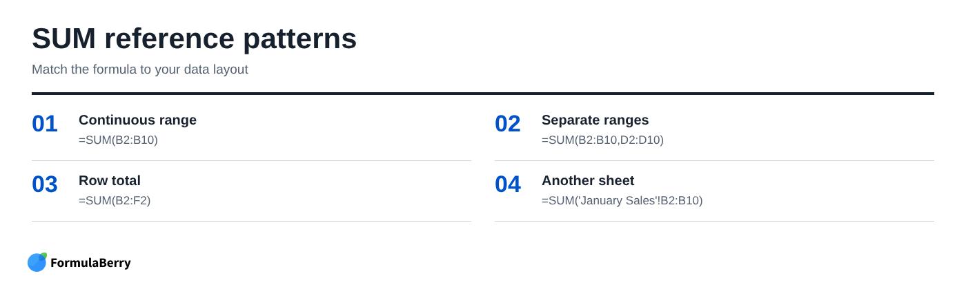
For monthly figures spread across columns, use a horizontal range. If January through May are in B2 through F2, enter:

=SUM(B2:F2)

This creates a row total for that product, employee, or account. If every row follows the same layout, drag the fill handle down to copy the formula to the rows below.

Add values from another sheet

To total values stored on a different tab, include the sheet name before the range:

=SUM(January!B2:B10)

If the sheet name contains spaces, wrap it in single quotes:

=SUM('January Sales'!B2:B10)

The source cells should contain actual numeric values for a meaningful total. A column of currency-looking text, for example, may need to be converted before SUM can add it correctly.

Use SUMIF when one condition controls what gets added

Use SUMIF when you only want to add values that match one rule. This is better than filtering the sheet manually and recalculating every time the data changes. For a related conditional function that counts matching text, numbers, or dates, see COUNTIF Formula in Google Sheets.

The pattern is:

=SUMIF(range_to_check, criterion, range_to_sum)

For example, if A2:A10 contains payment statuses and B2:B10 contains amounts, this formula adds only paid items:

=SUMIF(A2:A10,"Paid",B2:B10)

SUMIF checks each cell in column A for "Paid" and adds the corresponding value from column B.

Sum if a checkbox is checked

Checkboxes in Google Sheets evaluate as TRUE when checked and FALSE when unchecked. If column A contains checkboxes and column B contains amounts, use:

=SUMIF(A2:A10,TRUE,B2:B10)

This is useful for a budget where you want to total completed purchases, paid invoices, or approved reimbursements without moving rows to another section.

Sum if another cell contains text or does not contain text

Wildcards let SUMIF find text that appears within a longer cell value. To add amounts where the matching note contains the word "urgent," use:

=SUMIF(A2:A10,"*urgent*",B2:B10)

The asterisks mean that other text may appear before or after the word. For instance, "urgent - send today" and "review urgent request" both match.

To exclude rows containing a word such as "refund," use:

=SUMIF(A2:A10,"<>*refund*",B2:B10)

The <> operator means "not equal to." Do not use asterisks for an exact-text rule: "Paid" is the right criterion when the cell must equal Paid exactly.

Use SUMIFS for totals with multiple criteria

SUMIFS is the right choice when a total depends on two or more conditions. Unlike SUMIF, it starts with the range to add, followed by each criteria range and its matching criterion.

For example, you might want to total only approved Marketing expenses:

=SUMIFS(C2:C100,A2:A100,"Marketing",B2:B100,"Approved")

Here, column C holds amounts, column A holds categories, and column B holds statuses. SUMIFS adds a value only when the category is Marketing and the status is Approved.

That AND logic matters. SUMIFS does not add a row just because it meets one condition; every listed condition must be true.

Write a SUMIFS formula for a category and status

Build the formula in this order:

• Choose the numeric range to total: C2:C100.
• Add the first range to inspect: A2:A100, then its condition: "Marketing".
• Add the next range to inspect: B2:B100, then its condition: "Approved".

All ranges must cover matching rows and have the same dimensions. A common mistake is using C2:C100 as the sum range but A3:A100 as a criteria range. That shifts the rows out of alignment and produces an incorrect total.

The difference is straightforward: use SUMIF for one condition and SUMIFS for multiple conditions. Even if you only have one condition today, SUMIFS can be useful when you know you will add more filters later.

Avoid the mistakes that make SUM return the wrong total

When a total is wrong, do not immediately replace the formula. First verify what the formula is actually including and whether the source cells are numeric.

The most common problems are text stored as numbers, incomplete range endpoints, overlapping ranges, and totals placed inside their own source data.

Check whether numbers are stored as text

Imported data often looks numeric but is stored as text. It may have leading spaces, a leading apostrophe, or formatting inherited from another system. SUM can ignore these values, producing a total that seems too low.

Click a suspicious cell and inspect the formula bar. Remove leading apostrophes or spaces if present. When needed, convert a text value with:

=VALUE(B2)

You can also select valid numeric cells and use Format > Number to apply a number format. Formatting alone does not always convert text into a number, so test the result before relying on it in a total.

Prevent circular references and overlapping totals

A circular reference happens when a formula includes its own result cell, directly or through another formula. For example, =SUM(A2:A10) entered in A10 attempts to include A10 in the calculation.

Overlapping ranges can create a different kind of wrong result. Avoid =SUM(A2:A10,A8:A15) if rows A8:A10 should count only once, because those values are included twice. Use one non-overlapping range or revise the references so every row appears once.

Fix common Google Sheets SUM errors

Some SUM problems originate in the formula itself, while others come from a referenced cell. The fastest fix is to identify which situation you have before changing anything.

#VALUE!, #REF!, and circular dependency messages

#VALUE! usually means SUM is receiving an incompatible value or a referenced formula already has an error. Check the cells in the range for error messages or formulas that need correction.

#REF! means a reference is broken, often because a referenced row, column, or sheet was deleted. Edit the formula and restore the intended reference rather than rebuilding the total from memory.

A circular dependency message means the formula refers to itself directly or indirectly. Move the total outside the summed range, or adjust the range endpoint so it stops before the total cell.

A total of zero or a result that seems too low

A zero result can mean that cells that look like numbers are actually text. It can also mean your SUMIF or SUMIFS criterion does not match the source values exactly.

For totals that seem too low, check for an incomplete range such as =SUM(B2:B9) when the final amount is in B10. Click the formula cell and review the highlighted references in the sheet. This is often faster than reading a long formula character by character.

Make SUM formulas easier to maintain

Reliable totals come from simple structure. Put totals outside their source ranges, keep headers out of numeric ranges, and use one consistent data type in each amount column.

Open-ended ranges such as B2:B are convenient, but use them carefully. They can accidentally capture a future summary row placed lower in the same column. If your sheet includes subtotals and grand totals, use a defined range or place summary calculations in a separate column or section.

For recurring calculations, named ranges can improve readability. A formula such as =SUM(MonthlyExpenses) can be easier to audit than a long cell reference, but it is optional. A clearly organized sheet matters more than adding naming conventions to a small, one-off file.

Add reliable totals without rebuilding your spreadsheet

Use SUM for direct additions, SUMIF when one condition controls the total, and SUMIFS when every included row must meet multiple conditions. Keep the formula outside the source range, verify your selected references, and check that amounts are real numbers rather than text.

Those habits handle most Google Sheets total formulas without forcing you to reorganize an existing budget, report, or sales tracker.

FormulaBerry

If you know the result you need but are unsure how to write the formula, FormulaBerry can generate, explain, and help correct Google Sheets formulas from a plain-language request. For example, you can describe a need such as "sum approved Marketing expenses in column C" and use the generated formula as a starting point.

It is most useful for spreadsheet users who need formula help without memorizing function syntax. It is not a replacement for checking your ranges and source data: a correctly written SUMIFS formula can still return the wrong answer if the selected columns or criteria are wrong.