

The Google Sheets FILTER formula is simple until you add a second condition, a dropdown, imported text values, or an empty result. Then a formula that looked obvious can return #N/A, spill into the wrong area, or quietly include rows you did not want.
The good news is that FILTER is reliable once you understand how its conditions are evaluated. This guide shows how to build dynamic filters for text, dates, numbers, blanks, and multiple criteria without altering your original data.
What the FILTER function does in Google Sheets
FILTER returns only the rows or columns that meet one or more conditions. It leaves the source data unchanged and creates a separate, live result range wherever you enter the formula.
That distinction matters. The menu option under Data > Create a filter hides and shows rows within the existing table. The FILTER function produces a new table that updates automatically when source data or criteria change.
Imagine an orders table in columns A through D:
| Order ID | Region | Status | Amount |
|---|---|---|---|
| 1001 | West | Open | 450 |
| 1002 | East | Closed | 275 |
| 1003 | West | Open | 620 |
A FILTER formula can return only the West orders in another part of the sheet. The important rule is that each condition must line up with the range you are filtering. If you filter rows 2 through 100, every row-based condition must also cover rows 2 through 100.
Start with the FILTER syntax and a working example
The basic syntax is:
=FILTER(range, condition1, [condition2, ...])
range is the data you want returned. Each condition evaluates to a series of TRUE and FALSE results, one for each row or column. FILTER returns the entries where the required condition is TRUE.
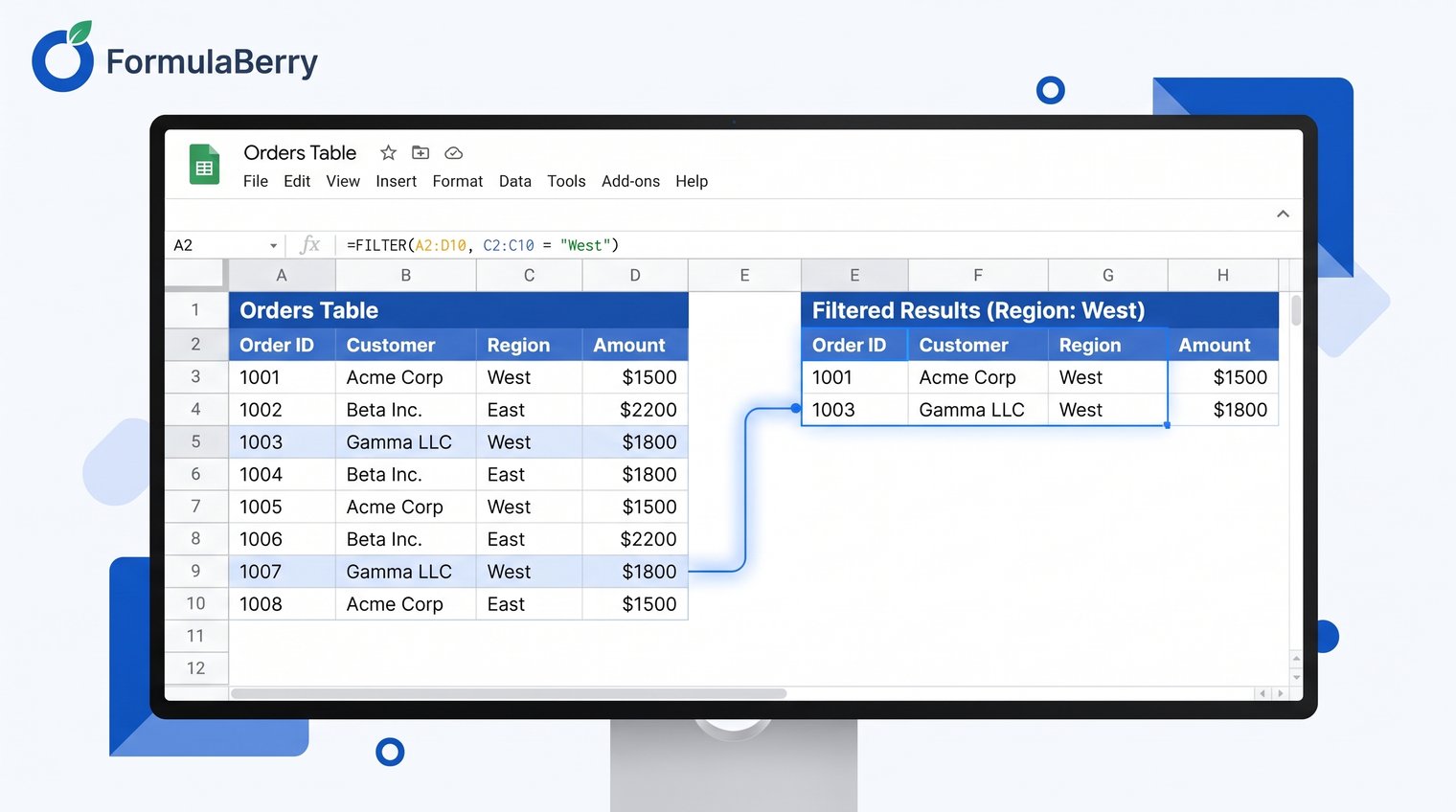
For the orders example, this formula returns every row where the Region in column B is West:
=FILTER(A2:D, B2:B="West")
Google Sheets evaluates B2:B="West" row by row. A West value produces TRUE; any other region produces FALSE. FILTER then returns the matching rows from A2:D.
You do not need to copy the formula down. FILTER spills its results into the cells below and beside the formula automatically, expanding or shrinking as the matching data changes.
Make the result dynamic with cell-based criteria
Hard-coding "West" is useful for a quick test, but a criteria cell makes the output reusable. Put a region name in G1, then use:
=FILTER(A2:D, B2:B=G1)
Now changing G1 from West to East changes the result instantly. G1 can be a typed value, but a data validation dropdown is usually the better choice because it prevents misspellings and inconsistent labels.
If you will copy the formula to another location, lock the criteria cell with an absolute reference:
=FILTER(A2:D, B2:B=$G$1)
An empty selector often creates confusing output. If G1 is blank, the formula may return records with blank regions instead of waiting for the user to choose a region. If you want no result until a selection is made, use:
=IF($G$1="", "", FILTER(A2:D, B2:B=$G$1))
Build a reusable filter formula template
For one required criterion, use this template:
=FILTER(data_range, criterion_range=criteria_cell)
For an optional criterion, allow all rows when the selector is blank:
=FILTER(A2:D, IF($G$1="", ROW(A2:A)>0, B2:B=$G$1))
The expression ROW(A2:A)>0 is TRUE for every row, so it effectively turns off that condition when G1 is empty. For more examples of using ROW to number rows and build references, see the Google Sheets ROW formula guide. Keep the data range and every condition range the same height. That is non-negotiable with FILTER.
Filter Google Sheets for specific text
For exact text matching, compare the source range directly to the text or criteria cell:
=FILTER(A2:D, C2:C="Open")
This is the right default for status labels, regions, categories, and other controlled values. It also handles values that look numeric but should remain text, such as product code 00125, provided the source values are stored consistently.
To find text contained anywhere in a cell, use SEARCH inside ISNUMBER. If G1 contains a word or phrase to look for in column C:
=IF(G1="", "", FILTER(A2:D, ISNUMBER(SEARCH(G1, C2:C))))
SEARCH returns a position when it finds the text and an error when it does not. ISNUMBER converts those results into the TRUE/FALSE array FILTER needs. SEARCH is not case-sensitive. Use FIND instead only if capitalization genuinely matters:
=FILTER(A2:D, ISNUMBER(FIND(G1, C2:C)))
Avoid false matches in text filters
Contains matching is broad by design. Searching for art will match both "art supplies" and "cart accessories." If you are filtering categories or statuses, exact matching is safer:
=FILTER(A2:D, C2:C=G1)
When you need to match a whole word in longer descriptions, REGEXMATCH can help:
=IF(G1="", "", FILTER(A2:D, REGEXMATCH(C2:C, "(?i)\b"&G1&"\b")))
The (?i) makes the match case-insensitive, and \b marks word boundaries. Do not use this for simple category fields; exact matching is easier to maintain. Also, do not place SEARCH directly in FILTER without ISNUMBER, because its no-match errors will break the condition.
Add multiple conditions with AND logic
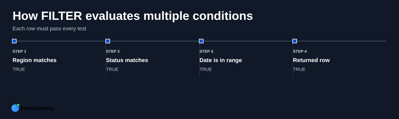
Separate conditions in FILTER use AND logic. Every returned row must pass every condition.
For example, to return orders where Region matches G1 and Status matches H1:
=FILTER(A2:D, B2:B=G1, C2:C=H1)
A row is returned only if both comparisons are TRUE. The same pattern works with dates and numbers. To return orders from a start date in G1 through an end date in H1:
=FILTER(A2:D, E2:E>=$G$1, E2:E<=$H$1)
This template assumes dates are in column E, separate from the Status column used earlier. Adjust the column references to match your actual layout. What matters is that each condition covers the same rows as the result range.
Use OR logic for multiple conditions in the same column
A frequent mistake is assuming commas create OR logic. They do not. Commas add separate FILTER conditions, which means AND.
To return orders from either East or West, add the two comparisons inside one condition:
=FILTER(A2:D, (B2:B="East")+(B2:B="West"))
Each comparison produces TRUE or FALSE values. Adding them creates 1 where one match is found, 2 where both tests would match, and 0 where neither matches. FILTER treats nonzero values as TRUE. The parentheses keep the OR group together.
For a longer allowed list, use MATCH. If accepted regions are listed in F2:F4:
=FILTER(A2:D, ISNUMBER(MATCH(B2:B, F2:F4, 0)))
This is easier to update than a long chain of added comparisons. For more ways to find positions and return values with MATCH, see the MATCH formula guide. Add or remove a region from F2:F4 without rewriting the formula.
Combine AND and OR conditions safely
Suppose you want East or West orders, but only those with an Open status. Put the OR group in one condition and the status test in a separate condition:
=FILTER(A2:D, (B2:B="East")+(B2:B="West"), C2:C="Open")
The first condition accepts either region. The second requires Open status. Without the parentheses around the OR expression, the formula is harder to read and easier to break when you add more logic.
Filter out blank rows and blank values
To remove blank rows from a live output, choose a column that should always contain a value for a valid record. If every order has an Order ID in column A:
=FILTER(A2:D, A2:A<>"")
This is especially useful when your source data is still growing. For a related approach, see this Google Sheets formula to filter out blank rows. You can combine it with another filter condition:
=FILTER(A2:D, A2:A<>"", B2:B=G1)
Use the column that defines a real record, not an optional field. For example, filtering on Status would incorrectly remove a valid order if Status is temporarily blank. If imported data contains cells with spaces, they are not technically blank. Use this test instead:
=FILTER(A2:D, LEN(TRIM(A2:A))>0)
Filter a dynamic range without pulling empty rows
Open-ended ranges such as A2:D are convenient because new rows are included automatically. But they can also bring empty rows into the output if your only condition can evaluate as TRUE for blanks.
The dependable pattern is an open-ended source range plus a nonblank key-column test:
=FILTER(A2:D, A2:A<>"", B2:B=G1)
This formula expands as data is added, but it ignores unfilled rows below the current dataset. Full-column references are practical for ordinary sheets, but they can slow recalculation in large workbooks with many array formulas. For a very large file, use a realistic bounded range such as A2:D5000 and extend it when needed.
Return useful results when no rows match
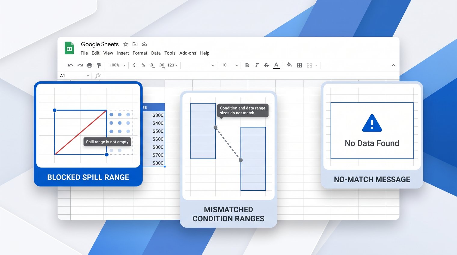
When FILTER finds no matching rows, Google Sheets returns #N/A. That does not automatically mean the formula is broken; it may simply mean no records meet the selected criteria.
Wrap the formula in IFNA to display a useful message instead:
=IFNA(FILTER(A2:D, B2:B=G1), "No matching records")
Use IFNA rather than IFERROR for this job. IFNA handles the expected no-results state while allowing genuine issues, such as an invalid range or a blocked spill area, to remain visible for debugging.
Fix the most common FILTER formula errors
Do not fix FILTER errors by randomly changing references until the message disappears. Start by checking the condition independently. In a spare column, enter a test such as =B2=G1 and fill it down. You should see TRUE only on rows that belong in the output.
Once a single condition works, add it to FILTER. Then add other conditions one at a time. This approach makes it clear which comparison, range, or data type is causing trouble.
Mismatched range sizes
The filtered range and every condition range must have matching dimensions. When filtering rows, they need the same number of rows.
This is a common mismatch:
=FILTER(A2:D100, B2:B99="West")
The data range contains 99 rows, while the condition contains 98. Align them:
=FILTER(A2:D100, B2:B100="West")
The same rule applies to open-ended ranges. Use A2:D with B2:B, not A2:D with B3:B.
Array result was not expanded
FILTER needs empty cells for its spill range. If text, values, or another formula already occupy cells where the results need to appear, Sheets reports that the array result was not expanded.
Clear only the obstructing cells, then let FILTER manage the output area. Do not place a FILTER formula inside a manually maintained table where someone is likely to type into the rows beneath it.
Dates and numbers that are stored as text
A value can look like a date or number while actually being text. That causes comparisons such as >=, <=, or exact numeric matches to fail unexpectedly.
Check a suspicious source value with:
=ISNUMBER(C2)
If it returns FALSE for a date or amount that should be numeric, correct or convert the source data. Changing the display format alone does not change text into a real number or date value.
Extend FILTER with sorting, unique results, and custom logic
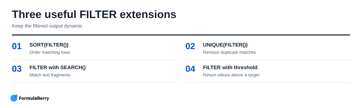
Once a base FILTER formula works, you can nest it inside other functions while keeping the result dynamic.
To sort matching rows by the fourth column in descending order:
=SORT(FILTER(A2:D, B2:B=G1), 4, FALSE)
To return a distinct list of matching values, such as unique customer names from column D:
=UNIQUE(FILTER(D2:D, B2:B=G1))
For a calculated condition, compare an amount column to a threshold stored in G1:
=FILTER(A2:D, D2:D>=$G$1)
You can also combine calculated tests with text criteria. For example, show Open orders above a target amount:
=FILTER(A2:D, C2:C="Open", D2:D>=$G$1)
These formulas remain live: a changed status, amount, or threshold updates the output without copying formulas or reapplying a menu filter.
A practical checklist for reliable Google Sheets FILTER formulas
- Choose an empty output area with enough room for the result to spill.
- Make the data range and every condition range start and end on matching rows.
- Start with one condition, verify it, then add more conditions gradually.
- Use separate condition arguments for AND logic.
- Use boolean addition or MATCH for OR logic in the same column.
- Use dropdown-driven criteria cells when other people will use the sheet.
- Add a nonblank key-column condition when filtering an expanding data range.
- Use IFNA when a no-match result is normal and should display a friendly message.
Most FILTER problems come down to range alignment, data types, or confusing AND with OR. Build the simplest version first and test each condition before nesting more logic around it.
If a condition is difficult to express, FormulaBerry can generate, explain, or help correct a Google Sheets FILTER formula from a plain-English description of the rows you want returned.