A spreadsheet can hold every number you need and still be hard to scan. When you are comparing monthly sales, project completion, website traffic, or budget changes across dozens of rows, a compact visual often tells the story faster than another column of figures.

Google Sheets sparklines solve that problem without adding separate chart objects. With one formula, you can place a tiny trend, progress bar, or column chart directly in a cell beside the data it summarizes.

What the SPARKLINE formula does in Google Sheets

The Google Sheets SPARKLINE formula creates a compact chart inside a single cell. Instead of building a full chart on top of your worksheet, you point the formula at a range and get an at-a-glance visual result in the formula cell.

This is especially useful for scanning row-by-row trends. A sales manager can see which products are rising or falling, a project lead can spot incomplete work, and a small business owner can review budget patterns without opening several full-size charts.

Google Sheets supports three main sparkline chart types:

• Line: Best for showing a trend over time.
• Bar: Best for showing one value against a target or maximum.
• Column: Best for comparing distinct periods or values, especially highs and lows.

A sparkline is a visual summary, not a replacement for the underlying numbers. It helps readers recognize a pattern quickly, but it is not designed for precise value reading.

Set up your data so each sparkline tells a clear story

Start with a layout that makes each row comparable. Put the item label in the first column, place dates or reporting periods across adjacent columns, and reserve one empty column at the end for the sparkline.

For example, a monthly sales report might use column A for product names, columns B through M for January through December sales, and column N for the trend chart. Each product then has one row of values and one matching sparkline.

Product	Jan	Feb	Mar	...	Dec	Trend
Product A	42	55	49	...	78	Line sparkline
Product B	64	58	71	...	62	Line sparkline

Keep periods in the same order for every row. If one row runs from January to December and another runs from December to January, the visuals may look valid but communicate opposite stories.

Also, use sparklines where pattern recognition matters more than exact labels. They work well in operational tables, scorecards, and recurring reports. They are less useful when readers need to identify the exact value for a specific day or month.

Create your first line sparkline

The basic syntax is:

=SPARKLINE(data, [options])

The data argument is the number or range you want to visualize. The optional options argument controls the chart type, colors, scale, and other display settings.

For a simple monthly trend in row 2, click the empty result cell, such as N2, and enter:

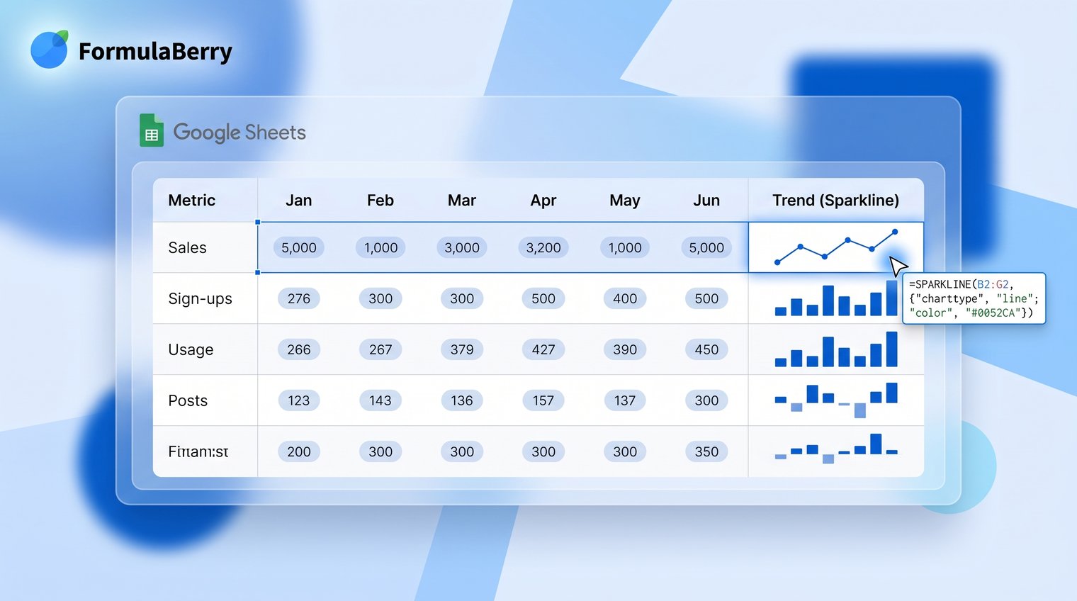
=SPARKLINE(B2:M2)

Press Enter. Google Sheets will create a line chart inside N2 using the values from B2 through M2. Once the first formula looks right, drag the fill handle down from the lower-right corner of N2 to apply it to the rest of the rows.

Use a basic trend example

Suppose row 2 contains monthly website visits: 1,200 in January, 1,450 in February, 1,310 in March, and so on through December. Entering =SPARKLINE(B2:M2) in the Trend column gives you an immediate view of whether traffic generally increased, declined, or fluctuated.

Line is the default chart type, so you do not need to specify it for a basic trend. This is the best starting point for a Google Sheets sparkline formula example because it lets you confirm that your source range is correct before adding styling options.

Use the options array to control chart type and appearance

After the basic formula works, you can customize it with an options array. In an options array, each setting is written as a property and value pair:

{"charttype","line";"color","#1a73e8"}

Use a comma between the property and its value, and use a semicolon to start the next option row. Add the array as the second argument in your formula:

=SPARKLINE(B2:M2,{"charttype","line";"color","#1a73e8"})

Google Sheets locales do not all use the same formula separators. If your sheet normally uses semicolons between function arguments, follow the separator pattern Google Sheets applies in your locale. Do not assume a copied formula is wrong until you check whether the issue is simply regional syntax.

Use options to make the chart easier to interpret, not to decorate a tiny cell. A readable color or a shared scale is useful; excessive styling is not.

Change the line color and thickness

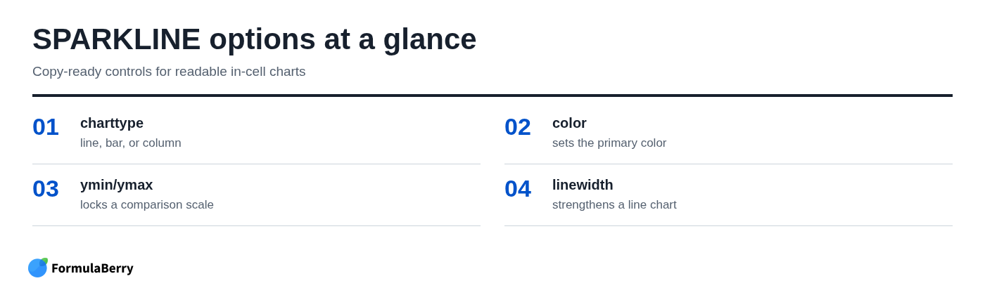
To make a line more visible, use the color and linewidth options:

=SPARKLINE(B2:M2,{"color","#1a73e8";"linewidth",2})

The hex color #1a73e8 produces a strong blue line, while linewidth set to 2 makes the trend easier to see in a narrow column. A thicker line is helpful when the row height is slightly larger or when values move only modestly. For a dense table with many rows, keep the line narrow enough that it does not look heavy.

Set a consistent scale across rows

By default, each line sparkline scales itself to the values in its own range. That makes each row visually prominent, but it can also mislead readers. A row that moves from 48 to 52 may look as dramatic as a row that moves from 10 to 90.

When comparing percentage scores, ratings, or any metric with a known shared range, set minimum and maximum values:

=SPARKLINE(B2:M2,{"ymin",0;"ymax",100})

Now every row is plotted on a 0 to 100 scale. This makes comparisons fairer across the table. The tradeoff is that subtle variation can become harder to see, so use a shared scale when relative size matters more than small within-row movement.

Create a bar sparkline for progress toward a goal

A bar sparkline is not primarily a trend chart. It is a compact progress indicator, ideal for completion percentages, budget usage, sales quota attainment, or inventory targets.

If C2 contains a completion percentage stored as a whole number from 0 to 100, use:

=SPARKLINE(C2,{"charttype","bar";"max",100;"color1","#34a853"})

The max option establishes the end of the bar's scale. In this example, a value of 75 in C2 fills 75 percent of the available bar width. The color1 option controls the filled portion of the bar.

Show remaining progress with a second color

Use color2 to show the unfilled portion of the target:

=SPARKLINE(C2,{"charttype","bar";"max",100;"color1","#34a853";"color2","#e8eaed"})

Green communicates completed progress, while the pale gray remainder makes the available target easy to see. This is usually clearer than showing a colored bar on a blank background.

Common mistake: the source value and max must use the same unit. If C2 contains 75, use "max",100. If C2 contains 0.75 because the cell is stored as a decimal percentage, use "max",1 instead. A mismatched maximum produces a bar that looks nearly empty or immediately full.

Create a column sparkline to compare periods

Use a column sparkline when individual periods should remain visually separate. This format is often easier than a line for spotting a standout month, an unusually weak week, or a large change in a category-based series.

For monthly values in B2 through M2, enter:

=SPARKLINE(B2:M2,{"charttype","column";"color","#4285f4"})

Each cell value becomes a separate vertical bar. The blue color keeps the chart simple and readable, but you can use a color that matches your existing report palette if it remains high contrast.

Highlight positive and negative values

Column sparklines are particularly useful for data that crosses zero, such as monthly profit and loss, variance from budget, or percentage change from the previous period. Use a second color for negative values and add an axis:

=SPARKLINE(B2:M2,{"charttype","column";"color","#34a853";"negcolor","#ea4335";"axis",TRUE})

Positive columns appear green and negative columns appear red. Setting axis to TRUE creates a baseline, which is important because readers need to see where positive performance ends and negative performance begins.

Without an axis, a loss and a small gain can be harder to distinguish in a tiny chart. For profit/loss reporting, budget variance, or other zero-centered measures, keep the axis on.

Copy sparklines down without breaking cell references

Build the formula once in the first result cell, then copy it down. If N2 contains =SPARKLINE(B2:M2), dragging the fill handle into N3 automatically changes the reference to B3:M3, then B4:M4, and so on.

This works because B2:M2 is a relative reference. For a report where every row uses its own series, relative references are the correct default.

If you need to apply a formula across a range rather than create one sparkline per row, an Array Formula in Google Sheets may be a better approach, depending on the structure of your sheet.

Use dollar signs only when part of a reference must remain fixed. For example, if a target is stored in cell P1 and you need it in another formula, use $P$1 to lock both the column and row. If only the column needs to stay fixed while rows change, use a reference such as $P2.

Once the results column is formula-filled, it updates automatically whenever the underlying source values change. There is no need to recreate the sparklines after each reporting cycle.

Handle blanks, text, and errors before they distort the chart

Sparklines depend on clean numeric input. Blank cells, text entries such as "N/A," and source errors can create confusing visuals or cause the formula to return an error.

If a row has no data yet, leave the sparkline cell blank rather than showing an empty chart. This wrapper checks whether the source range contains anything before creating the sparkline:

=IF(COUNTA(B2:M2)=0,"",SPARKLINE(B2:M2))

For criteria-based checks elsewhere in a report, the COUNTIF Formula in Google Sheets can help identify text, numbers, or dates that meet a condition before you visualize the results.

For reporting, fix source errors whenever possible. An error in a sales total or budget calculation should be investigated rather than hidden just so the sparkline renders. Error-handling wrappers can be useful when a blank is a meaningful reporting choice, but they should not mask a broken calculation.

Also standardize entries before visualizing them. A mixture of numbers, percentage text, dashes, and manually typed notes in the same range is a data-cleaning problem, not a sparkline formatting problem.

Avoid the most common SPARKLINE formula mistakes

Most SPARKLINE issues come down to syntax, scale, or using the wrong chart type for the question.

• Malformed options arrays: Option names and text values need quotation marks. Write "charttype","column", not charttype,column. Also check whether your Google Sheets locale requires different separators.
• Misleading autoscaling: Rows can look equally volatile even when their value ranges are very different. Use ymin and ymax when a common baseline is necessary.
• Incorrect bar maximum: A value of 0.82 requires a maximum of 1 for an 82 percent bar. A value of 82 requires a maximum of 100.
• Too much data in too little space: A 100-point daily series squeezed into a narrow cell may create visual noise rather than insight. Aggregate to weekly or monthly values, widen the column, or use a standard chart.
• Using visual color without meaning: If red means negative values in one column and merely "important" in another, readers have to decode the report repeatedly. Keep color meanings consistent.

Know when a sparkline is the wrong chart

Sparklines are deliberately minimal. They do not provide detailed axis labels, data labels, robust annotations, or interactive exploration. That is their strength in a compact table, but it is also their limit.

Use sparklines when a reader needs to compare many rows at a glance: which product is trending up, which department is under target, or which project is approaching completion. Use a standard Google Sheets chart when the reader needs labeled axes, multiple series, exact values, annotations, or a visual intended for a stakeholder presentation.

A simple decision rule works well: if the table provides the detail and the chart only needs to reveal the pattern, choose a sparkline. If the chart itself must carry the explanation, build a full chart.

Build a readable sparkline dashboard

A useful sparkline dashboard starts with comparable rows and consistently ordered periods. Choose a line sparkline for trends, a bar sparkline for progress toward a defined maximum, and a column sparkline when individual periods or positive-versus-negative movement matter.

Start with one copy-ready formula, then add only the options that improve interpretation. A shared scale may make comparisons more honest. A high-contrast color may make a dense table easier to scan. Beyond that, keep the in-cell chart simple.

If you need help turning a reporting requirement into the right Excel or Google Sheets formula, FormulaBerry can generate, explain, and help correct formulas from a plain-language request. You can also use its Google Sheets Formula Generator for a more specific formula request.