
An inconsistent formula warning in Excel is easy to dismiss, especially when the number in the cell looks reasonable. That is how small spreadsheet mistakes survive: one row uses the wrong range, misses an IF condition, or points to last month's rate while every other row follows a different pattern.
The warning does not automatically mean Excel has found a wrong answer. It means Excel has noticed a formula that differs from nearby formulas in a region that appears to follow a pattern. The right response is not "always fix it" or "always ignore it." It is to verify the logic before changing anything.
What an Inconsistent Formula Warning Means in Excel
Excel raises an inconsistent formula warning when a formula in one cell does not match the pattern of surrounding formulas. You will usually see a small green triangle in the upper-left corner of the cell, followed by a warning button when you select it.
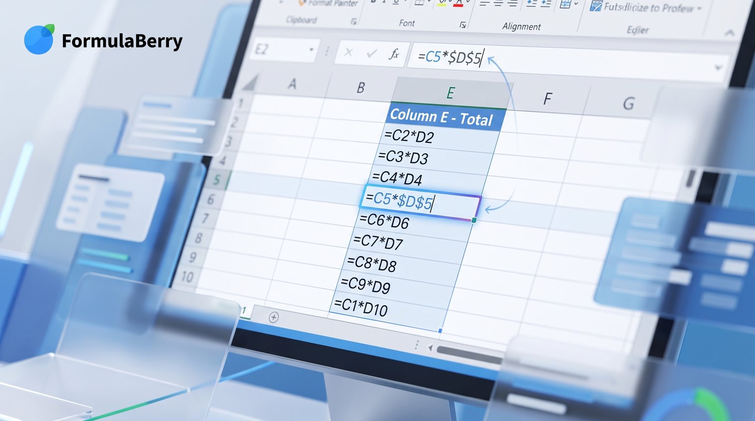
For example, if cells D2 through D10 contain formulas that multiply the values in columns B and C, Excel expects each row to follow that same reference pattern. If D6 contains =B6*C5 while the rows around it use =B5*C5, =B7*C7, and so on, Excel flags D6 because its references break the sequence.
This often happens after copying formulas, manually editing a row, inserting a new row, or pasting values over formulas. It can also appear in a worksheet where a single exception is entirely deliberate, such as a subtotal, adjustment, or row with a different pricing rule.
Decide Whether the Formula Is Actually Wrong Before You Change It
Start by comparing the flagged formula with the cells immediately above and below it. Select the warning cell, then look at the formula bar. Check whether the row references advance in the same way as the neighboring formulas.
Suppose column E calculates sales tax:
| Row | Formula |
|---|---|
| E5 | =D5*$B$1 |
| E6 | =D6*$B$1 |
| E7 | =D7*$B$1 |
If E6 instead contains =D6*$B$2, it may be incorrect. But if row 6 is a special tax-exempt transaction and B2 stores a zero tax rate, the difference is intentional. Excel recognizes a pattern difference, not your business rules.
Pause before copying a neighboring formula over the cell when the row is any of the following:
- A subtotal, total, or grand total row
- A manually entered adjustment or credit
- A blank-source row that should return an empty result
- A row governed by a different commission, tax, or discount rule
- A calculation that intentionally uses a fixed reference cell
The common mistake is treating every green triangle as an error and overwriting a valid exception. Check the row label, source data, and intended calculation first.
Open Excel's Error-Checking Options and Inspect the Flagged Cell
Select the cell with the green triangle. Excel displays a yellow warning button beside it. Click that button to see the message, which may read "Inconsistent formula" or "Inconsistent calculated column formula."
The menu gives you several actions. Read the message before choosing one:
- Help on this error is useful when you need Excel's explanation of the warning category.
- Trace Error helps identify the cells feeding into the formula and can expose a shifted or missing reference.
- Edit in Formula Bar is the safest choice when you already know which part of the formula needs correction.
- Ignore Error removes the warning for that cell, but it does not validate the formula or repair anything.
Do not choose a suggested action simply because it is available. Excel cannot tell whether a different formula reflects a mistake or an intentional exception in your workbook.
Use Trace Error to Find the Inputs Behind the Result
Choose Trace Error when the formula looks almost right but produces an unexpected result. Excel draws arrows between the selected formula and its precedent cells, making it easier to spot a reference that points to the wrong row, sheet, or range.
You can also use the Formulas tab and select Trace Precedents to see inputs, or Trace Dependents to see which later calculations rely on the selected cell. This is particularly useful when a formula was copied across columns and one reference moved when it should have stayed fixed.
For instance, a monthly report might use =SUM(B2:B31) in one total cell but accidentally use =SUM(C2:C30) in another. The formula is valid, yet the arrows and highlighted ranges reveal that one day or one column has been omitted.
Compare the Formulas, Not Just the Displayed Values
Displayed values can hide formula errors. Two different formulas may both show $500 today, then produce different results when the source data changes. Always inspect the formula pattern itself.
Click a formula cell and review the formula bar, then compare it to the cells above and below. For a larger inconsistent formula Excel column, press Ctrl+` to turn on Show Formulas. The grave accent key is usually located below Esc or to the left of the number 1 key. Press the shortcut again to return to normal values.
With formulas visible, scan for differences in references, operators, function names, and ranges. Pay special attention to these patterns:
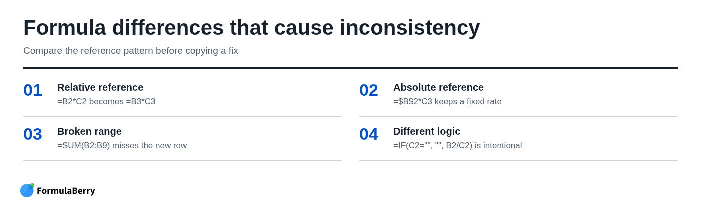
- Relative references change when copied. =B2*C2 should become =B3*C3 on the next row.
- Absolute references stay fixed. =$B$2*C3 always uses the value in B2 while C3 changes by row.
- Mixed references lock either a column or row, such as =$B3 or =B$3.
- Ranges can stop too early after an inserted row, such as =SUM(B2:B9) when the intended range now runs through B10.
Fix a Single Formula Without Breaking Its References
When only one formula is wrong, edit that cell rather than filling an entire column. Select the cell, press F2 or click in the formula bar, and correct the operator, function, range, or reference that differs from the intended pattern. If you need help reconstructing or checking the expression, see this guide to Excel formula assistance.
For example, if a margin formula should be =(C12-B12)/C12 but reads =(C12-B12)/B12, replace only the final reference. Then compare it with the neighboring formulas and ask whether the result is plausible for that row.
Do not validate a correction based only on the disappearance of the green triangle. A formula can match its neighbors and still be logically wrong if the entire formula block was copied incorrectly. Check the inputs, the formula, and the resulting number.
Correct Relative, Absolute, and Mixed References
A missing or misplaced dollar sign changes how a formula behaves when you copy it. This is one of the most common causes of an inconsistent formula Excel warning after filling a range.
Imagine cell E2 calculates tax using the amount in D2 and a tax rate stored in B1. The correct formula is =D2*$B$1. When copied down, it becomes =D3*$B$1, =D4*$B$1, and so on. The transaction amount changes by row; the tax rate does not.
While editing a reference, press F4 to cycle through reference types: B1, $B$1, B$1, and $B1. Choose the form that matches what should move when the formula is copied. On some laptops, you may need to press Fn+F4.
A lookup table is another common example. If your formula needs to search a fixed range such as H2:I20, use $H$2:$I$20 so the lookup range does not slide down one row every time you fill the formula.
Restore a Consistent Formula Down a Column
Once you have verified the correct formula pattern, repair the affected range using a formula you trust. Copying a verified adjacent formula is usually the safest starting point because Excel adjusts relative references automatically.
Use one of these methods depending on the worksheet:
- Copy and paste: Copy a correct formula cell, select the cells that should follow the pattern, and paste.
- Fill handle: Drag the small square at the lower-right corner of a correct cell down through the target rows.
- Double-click the fill handle: Use this when an adjacent column contains continuous data. Excel fills down to the end of that nearby data block.
- Fill Down: Select the correct formula plus the cells below it, then press Ctrl+D.
Autofill formula behavior is convenient, but it is not a substitute for review. Excel may fill through a subtotal row, a blank separator, or an exception row that needs different logic. After filling, use Show Formulas and inspect the first, last, and a few middle rows.
Repair a Calculated Column in an Excel Table
In an Excel Table, a formula entered in one row commonly becomes a calculated column formula. Excel may offer to apply that formula to every row in the table, which is useful when the column should use one consistent rule.
To fix an inconsistent calculated column formula in Excel, enter the correct formula in a cell within the affected table column. Review Excel's proposed propagation before accepting it. If the formula should apply to all standard rows, allow Excel to update the calculated column. If some rows intentionally use different logic, keep those exceptions and make them obvious with labels or notes.
Structured references make table formulas easier to read. A formula such as =[@Quantity]*[@UnitPrice] clearly indicates that it multiplies values from the current row, which reduces the chance of accidentally referencing the wrong row number.
FormulaBerry

When you know the result you need but cannot reconstruct the correct formula, FormulaBerry can help translate the intended calculation into an Excel or Google Sheets formula. For example, you could describe: "Return blank if C2 is empty; otherwise divide B2 by C2 and round to two decimals." That is more reliable than guessing at nested IF logic. An Excel formula generator can be useful for turning that plain-language description into a starting formula.
It is also useful for explaining a formula you inherited, especially one containing fixed references, lookups, or multiple conditions. The limitation is important: FormulaBerry can generate, explain, and help correct formulas, but it cannot determine your business rule without a clear description. You still need to confirm which rows are exceptions and what the calculation should do.
Find Formula Inconsistencies Across a Larger Worksheet
For a large worksheet, do not assume every formula in every column should match. Divide the sheet into logical blocks first: detail rows, subtotals, summary sections, input areas, and calculations often have different rules.
Use Home > Find & Select > Go To Special > Formulas to select formula cells in the active sheet. Then turn on Show Formulas with Ctrl+` and inspect each formula block for breaks in the expected pattern.
Filtering can help isolate categories, departments, or date ranges that should use the same calculation. Sorting can also reveal anomalies, but use caution: sort the entire data range or Excel Table, not only the formula column. Sorting a single column can detach formulas from the records they belong to.
For an inconsistent formula Excel multiple column problem, check each calculation column separately. A revenue column, a tax column, and a margin column may all have valid but different formula patterns. The goal is consistency within a logical formula region, not forced uniformity across the whole worksheet.
Use Excel's Formula Auditing Tools for Hard-to-Spot Errors
Pattern checks identify formulas that look different. Formula auditing tools help you understand why a formula calculates the way it does.
- Error Checking moves through formula warnings and lets you inspect each one.
- Evaluate Formula calculates a formula step by step, which is useful for nested IF statements, lookups, and long expressions.
- Watch Window keeps selected cells visible while you work elsewhere in a large workbook.
- Trace Precedents and Trace Dependents reveal source cells and downstream effects.
Use these tools selectively. A green triangle may identify the odd formula, while Evaluate Formula tells you whether that odd formula actually returns the intended result.
Handle the Most Common Causes of Inconsistent Formulas
Most inconsistent formulas come from a handful of repeatable spreadsheet mistakes. Fix the underlying cause rather than only clearing the warning.
| Cause | What to check | Typical fix |
|---|---|---|
| Copied formula with shifted references | Row, column, and lookup-range references | Correct relative or absolute references, then refill the affected range. |
| Row inserted inside totals | Whether the SUM or other range includes the new row | Extend the range or use a Table so totals expand more reliably. |
| Formula replaced with a value | Whether one cell contains a hard-coded number | Restore the formula unless the override is intentional and documented. |
| Omitted IF condition | Blank, zero, or error-handling logic in nearby rows | Restore the condition, such as returning blank when a source cell is empty. |
| Inconsistent table formula | Whether the calculated column should apply to all rows | Apply the correct table formula or preserve a clearly labeled exception. |
Also distinguish the inconsistent formula warning from formula errors such as #REF!, #DIV/0!, and #VALUE!. An inconsistent formula can return a normal-looking number. By contrast, those error values indicate a specific problem with a reference, division, or data type. Fix the underlying reference or source-data issue first, then review whether the formula pattern is still consistent.
When Ignoring the Warning Is the Correct Choice
Ignoring the warning is appropriate when the different formula is deliberate, verified, and understandable to the next person who opens the workbook. A subtotal that uses =SUM(D2:D10) should not be forced to match detail-row formulas such as =B2*C2.
Before selecting Ignore Error, confirm the calculation and document the exception. Add a clear label such as "Subtotal," "Manual Adjustment," or "Tax Exempt." If the sheet is used regularly, add a note or visually separate the exception row from standard data rows.
Ignoring the warning without context is not cleanup. It removes a useful signal and makes future spreadsheet maintenance harder.
Prevent Inconsistent Formulas in Future Workbooks
The best fix is a workbook design that makes accidental differences less likely. Convert repeating data ranges into Excel Tables, use structured references where practical, and keep assumptions such as tax rates, exchange rates, and lookup lists in clearly labeled locations.
Protect formula cells in shared workbooks so users can enter data without overwriting calculations. Keep input cells visually distinct from calculated cells, and separate totals from detail rows instead of inserting totals into the middle of a data block.
After adding rows or columns, audit the affected formulas before distributing the workbook. Test copied formulas on a few representative rows: one normal record, one blank or zero-value case, and one record near the end of the range. This catches reference drift before it spreads through an entire report.
A Reliable Final Check Before You Dismiss the Warning
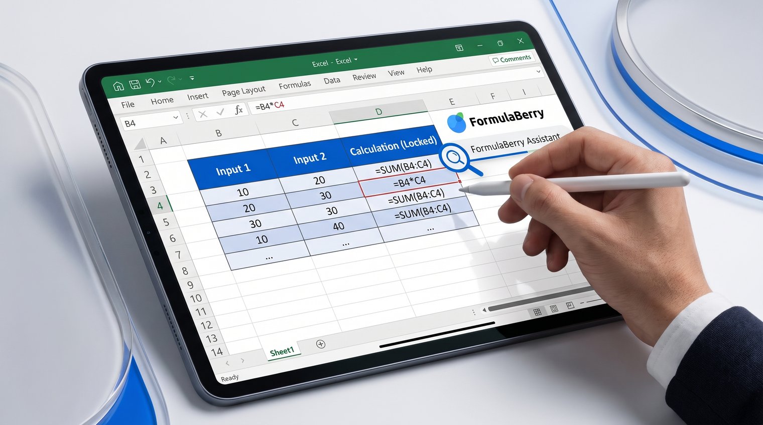
Use a simple sequence whenever Excel flags an inconsistent formula: compare the neighboring formulas, confirm the references and ranges, trace inputs if something is unclear, and validate whether the result makes sense for that row. Then either correct the formula or intentionally ignore the warning with a clear reason.
That short review is far safer than blindly filling a formula down a column or dismissing every green triangle. If the intended calculation is unclear, FormulaBerry can help you generate, explain, or correct the Excel formula from a plain-language description.