IRR is easy to calculate in Excel and surprisingly easy to misread. The biggest mistakes are using IRR on irregular dates, treating a monthly result as an annual return, or building a cash-flow range in the wrong order.

Use the right function, lay out the cash flows chronologically, and check what period each value represents. Then Excel can calculate a return rate that is useful for comparing a project, investment, or purchase decision against your required rate of return.

Use Excel's IRR formula for regularly spaced cash flows

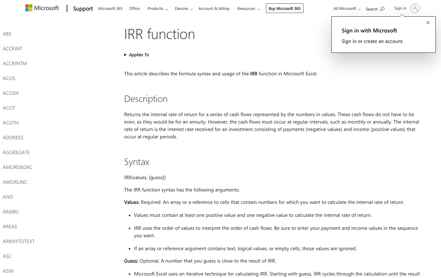
Excel's IRR function calculates the periodic return for a set of cash flows that occur at equal intervals. Those intervals can be years, quarters, or months, but they must be consistent.

The syntax is:

=IRR(values, [guess])

• values is the range containing your cash flows, including the initial investment and later income or proceeds.
• guess is an optional starting estimate for the return rate. Most of the time, you can leave it out.

IRR returns a rate per period. If each value represents one year, the result is an annual IRR. If each value represents one month, the result is a monthly IRR, not an annual percentage.

Set up the cash-flow range correctly before calculating IRR

Your range needs at least one negative cash flow and at least one positive cash flow. In a typical investment model, the first value is the cash paid out, shown as a negative number, followed by the cash received in later periods.

For example, a project costing $10,000 today with annual returns over the next four years could look like this:

Period	Cash flow
Year 0	-$10,000
Year 1	$2,500
Year 2	$3,000
Year 3	$3,500
Year 4	$4,000

Enter a zero when a complete period has no cash flow. Do not remove that period from a monthly or quarterly series just because nothing happened; deleting it changes the time spacing Excel assumes.

IRR uses position, not labels, to determine timing. Whether the values run down a column or across a row does not matter, but they must appear in chronological order.

Calculate IRR in Excel with a worked example

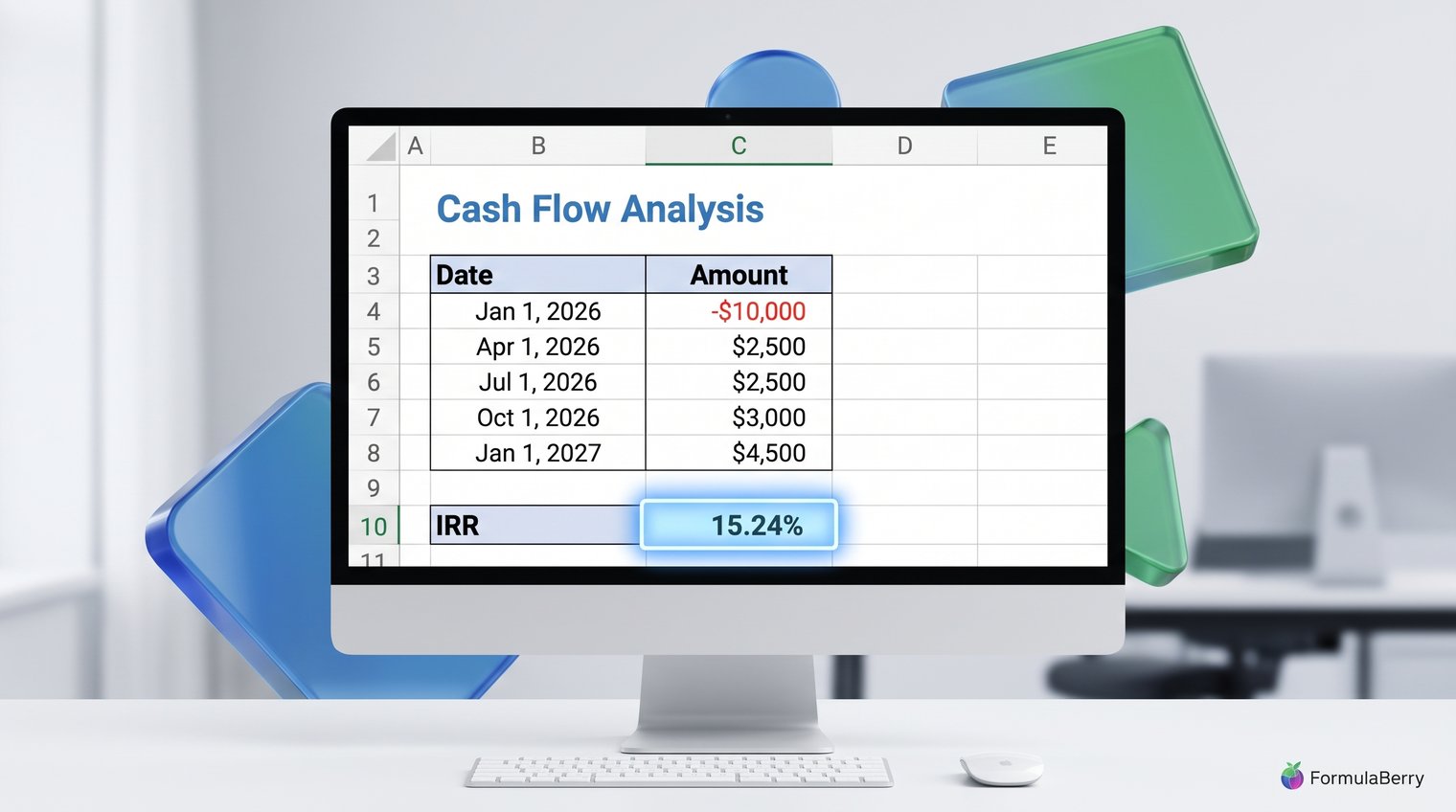
Suppose the cash flows in the table are entered in cells B2 through B6. Click the cell where you want the result and enter:

=IRR(B2:B6)

Press Enter, then format the result cell as a percentage. For analysis, keep at least two decimal places rather than rounding immediately to a whole number. For related percentage calculations, see this Excel percentage formula guide.

Excel will calculate the discount rate at which the value of future cash inflows offsets the initial cash outflow. If the displayed result is about 10%, that means the project has an annual IRR of about 10% because the values represent annual periods.

Example: annual project cash flows

Using the same annual cash flows in B2:B6, Excel treats B2 as Year 0 and each later cell as the next annual period.

With those figures in B2:B6, use =IRR(B2:B6). Excel is effectively finding the rate that makes the net present value of all five cash flows equal zero.

A 12% IRR, for example, means the cash-flow sequence produces an estimated annual return of 12% when each period is one year. It does not mean the project earns exactly 12% in every individual year.

Use the guess argument only when Excel needs help converging

When you omit the optional guess, Excel starts with an estimate of 10%. That is usually enough for ordinary cash-flow patterns, so =IRR(B2:B6) is the best default.

If Excel cannot find a result, supply a reasonable starting estimate. For example:

=IRR(B2:B6,0.15)

Here, 0.15 tells Excel to begin its search near 15%. It is not a target return and does not force the answer to be 15%.

Try another plausible guess when your cash flows switch from negative to positive more than once. A pattern such as negative, positive, negative can have multiple valid IRRs, and the guess may influence which result Excel returns.

Calculate monthly cash-flow IRR and annualize it correctly

If each value represents one month, Excel's IRR formula returns a monthly rate. For 12 monthly values in B2:B13, use:

=IRR(B2:B13)

To convert that monthly rate into a compounded annual return, use:

=(1+IRR(B2:B13))^12-1

Do not simply multiply the monthly IRR by 12 unless you only need a rough, non-compounded approximation. The compounded formula assumes the monthly rate applies consistently across 12 months; compounding is the more accurate annualized rate in that case.

A common mistake is annualizing a result when the cash flows are not actually monthly. If some payments are delayed, skipped, or made on arbitrary dates, use XIRR instead. IRR only works cleanly when every position in the range represents the same length of time.

Use XIRR instead when cash-flow dates are irregular

IRR assumes equal time intervals. Real projects and investments often do not behave that neatly: a deposit may be made on January 15, a payment received on April 3, and a final amount received late in December. In those cases, XIRR is the better function.

The syntax is:

=XIRR(values, dates, [guess])

For working with the date values used by XIRR, see this Excel date formula guide. If cash flows are in B2:B5 and their actual dates are in A2:A5, enter:

=XIRR(B2:B5,A2:A5)

XIRR uses the dates to account for the actual number of days between transactions. Its result is annualized, so do not multiply it by 12 or apply another annualization formula.

When IRR is still the right function

Use IRR when the periods are genuinely even: one value every month, quarter, or year. The cash flows can be arranged vertically or horizontally, as long as each adjacent cell represents the next complete period.

For instance, a monthly operating forecast with one row for January through December is a good IRR use case, even if the entries are in columns rather than a vertical range.

When XIRR gives a more reliable answer

Use XIRR when transactions occur on different calendar dates, a payment period is skipped, or a project begins and ends mid-month or mid-year. It is generally the more realistic choice for investment records and transaction-based project models.

Make sure the dates range and values range contain the same number of cells and remain aligned. The date in A2 must describe the cash flow in B2, the date in A3 must describe B3, and so on.

Understand how Excel calculates IRR

Excel calculates IRR by searching for the rate that makes the present value of all your cash flows add up to zero. Put simply, it asks: at what return rate is the initial amount paid out exactly balanced by the value of money received later?

Earlier cash inflows generally improve IRR because they are received sooner. Delayed inflows reduce it. The size and order of negative and positive values matter just as much as the total amount received.

IRR is therefore a calculation based on your assumptions, not a guarantee of investment performance. If future cash flows are estimates, the IRR is also an estimate.

Fix #NUM!, #VALUE!, and misleading IRR results

Before changing formulas, run three quick checks: confirm every input is numeric, confirm the range contains both positive and negative values, and confirm the values are in chronological order. Those checks solve a large share of IRR problems.

Fix #NUM! errors

#NUM! commonly appears when there is no sign change in the values, Excel cannot converge on a result, or the cash-flow pattern has no usable IRR.

• Check that at least one value is negative and at least one is positive.
• Verify that the initial investment has not been entered as a positive number by mistake.
• Try a reasonable guess, such as =IRR(B2:B6,0.10) or =IRR(B2:B6,0.25).
• Use XIRR if the values are not evenly spaced in time.

Do not use a wildly high or low guess just to remove the error. First make sure the cash-flow model represents a real, internally consistent sequence.

Fix #VALUE! errors

#VALUE! usually means there is text, an existing formula error, or an invalid reference in the values range. Check for entries such as "N/A," dollar signs typed directly into cells, blank-looking text values, or formulas that return errors.

With XIRR, also verify that every date is a valid Excel date and that the values and dates ranges have exactly the same number of cells. A mismatched range such as B2:B6 paired with A2:A5 will not work.

Watch for multiple IRRs and unrealistic rates

More than one switch between negative and positive cash flows can create multiple IRRs. For example, an investment with an initial outlay, an inflow, and a later cleanup cost may produce different answers depending on the guess argument.

Even a mathematically valid IRR can be misleading when comparing mutually exclusive projects of very different sizes or timing. Use net present value alongside IRR, and consider a modified return measure when cash flows are unconventional.

Validate the result before using it in a decision

Compare IRR with your hurdle rate, financing cost, or required return only after confirming the period basis. A 2% monthly IRR and a 2% annual IRR are not remotely equivalent, even though they display the same percentage.

For regularly spaced periods, you can verify an IRR result with Excel's NPV function:

=NPV(rate, future_cash_flows)+initial_cash_flow

For the earlier example, where the initial outlay is in B2 and future inflows are in B3:B6, a check could be:

=NPV(IRR(B2:B6),B3:B6)+B2

The result should be very close to zero. Excel's NPV function treats the first value in its range as occurring one period from now, which is why the time-zero initial investment belongs outside the NPV range.

Do not choose a project based on IRR alone. Review NPV, investment size, when cash arrives, the reliability of the forecast, and the risk of the project.

Use clear formula prompts when you need help building or explaining IRR calculations

If the issue is translating your model into the right formula, describe the layout and timing clearly. Useful requests include:

• "Create an Excel formula for monthly IRR using cash flows in B2:B13 and annualize the result."
• "Write an XIRR formula for values in C2:C10 and dates in B2:B10."
• "Explain why my IRR formula returns #NUM! when my first value is -5000."
• "Correct this formula so it calculates return using irregular payment dates."

FormulaBerry's Excel formula generator can generate, explain, and help correct Excel and Google Sheets formulas from a plain-language request. Include your cell ranges, whether the periods are monthly or annual, and whether you have actual dates for the most useful answer.

Choose IRR or XIRR based on your cash-flow timing

Use IRR when your cash flows occur at equal intervals. Use XIRR when actual transaction dates are irregular. That one decision prevents many incorrect return calculations.

Before trusting either result, make sure the model includes both positive and negative cash flows, preserves chronological order, and uses the correct period interpretation. If you need help building or troubleshooting the formula behind a cash-flow model, FormulaBerry can help turn the setup into the right Excel or Google Sheets formula.