
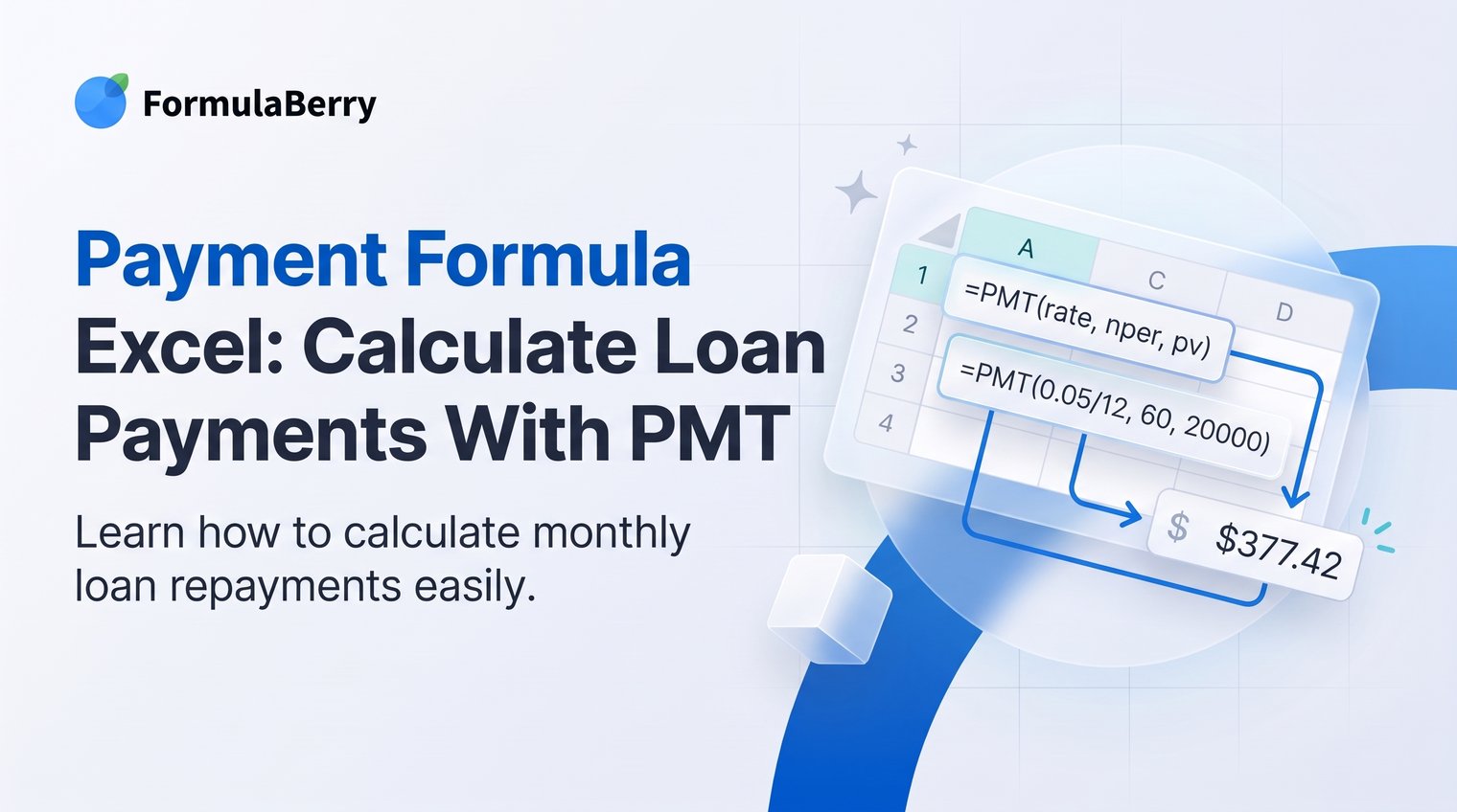
A loan payment can look deceptively simple until a spreadsheet returns a negative number, a payment that is far too low, or an error you cannot explain. In most cases, the issue is not Excel. It is a mismatch between the interest-rate period and the number of payments.
Excel's PMT function handles the math for fixed-rate loans with equal payments, including mortgages, car loans, and personal loans. Once your inputs are set up correctly, you can calculate a dependable monthly payment in one formula and use it as the foundation for a loan comparison or amortization schedule.
Use Excel's PMT Formula for a Monthly Loan Payment
Use PMT when a loan has a fixed interest rate and regular, equal payments. It returns the payment required each period to pay a loan down to its expected ending balance, usually zero.
The basic syntax is:
=PMT(rate, nper, pv, [fv], [type])
For a straightforward monthly loan payment, you might use:
=PMT(6.5%/12,30*12,-250000)
This calculates the monthly payment for a $250,000 loan at 6.5% interest over 30 years. Excel normally follows cash-flow signs: money received is positive and money paid is negative. If you enter a positive loan amount, PMT commonly returns a negative payment. Using a minus sign before the loan amount is the clearest way to display the payment as a positive currency amount.

Set Up the Loan Inputs Before Writing the Formula
Do not bury loan assumptions inside a long formula if you expect to change them later. Put each input in a labeled cell so you can audit the calculation, compare scenarios, and immediately see what changed.
For example, create a small input table like this:
| Cell | Label | Value |
|---|---|---|
| B2 | Annual interest rate | 6.5% |
| B3 | Loan term in years | 30 |
| B4 | Loan amount | $250,000 |
Format B2 as a percentage, B4 as currency, and B3 as a general number. This setup is more useful than a hard-coded formula because you can test a different down payment, rate, or term without rebuilding the calculation.
Keep the values as true numbers. A cell containing "$250,000" entered as text, for example, can trigger an error even though it looks like a valid amount on screen.
Convert the Annual Rate and Loan Term to Monthly Values
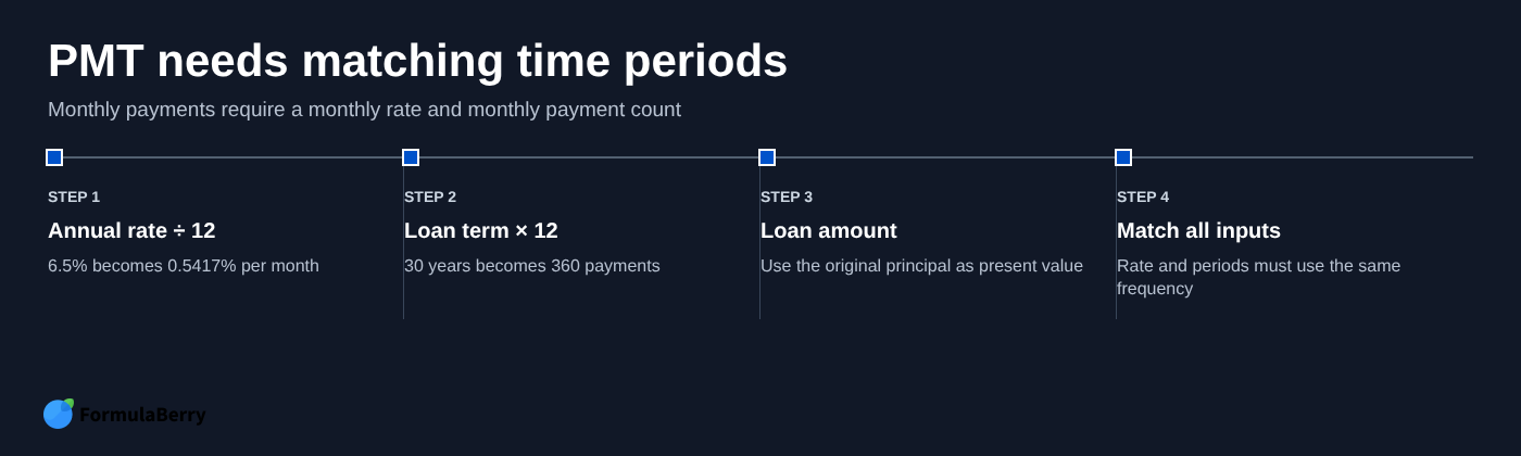
A monthly payment formula requires monthly inputs. That means you must convert the annual interest rate into a monthly rate and the loan term in years into the total number of monthly payments.
With the example cells above:
- Monthly interest rate: B2/12
- Total monthly payments: B3*12
- Present value, or amount borrowed: B4
A 6.5% annual rate becomes approximately 0.5417% per month, and a 30-year term becomes 360 monthly payments. Excel can perform both conversions inside PMT, so you do not need extra helper cells unless you want them.
The most common mistake is using an annual rate with a monthly payment count. For example, =PMT(B2,B3*12,-B4) is wrong because B2 is annual while the number of periods is monthly. The rate and period count must always use the same frequency.
Enter the Monthly Payment Formula in Excel
Click the cell where you want the monthly payment to appear and enter:
=PMT(B2/12,B3*12,-B4)
Based on the sample layout, Excel divides the annual rate in B2 by 12, multiplies the years in B3 by 12, and uses the amount in B4 as the loan principal. The minus sign before B4 makes the result display as a positive payment.
If you prefer to test the formula with fixed values first, use:
=PMT(6.5%/12,30*12,-250000)
The result is roughly $1,580 per month before property taxes, homeowners insurance, lender fees, and other costs that may appear in a real mortgage payment.
Understand Each PMT Argument
The first three PMT arguments do nearly all the work for standard loans:
- rate: Interest rate for one payment period. For monthly payments, use the annual rate divided by 12.
- nper: Total number of payment periods. For a 30-year monthly loan, use 30 times 12.
- pv: Present value, or the amount borrowed today. Enter it as a negative value if you want PMT to return a positive payment. For related present-value calculations, see this PV Formula Excel guide.
The optional fv argument is the balance you want left after the final payment. Most fully amortizing loans end at zero, so you can omit it. The optional type argument controls payment timing: use 0, or omit it, for payments at the end of each period. That is the normal setting for most loans.
Format the Result as Currency
After entering the formula, format the payment cell as Currency or Accounting with two decimal places. In Excel, select the cell, open the Number Format menu, and choose Currency or Accounting.
Do not mistake the PMT result for your full lender bill. PMT calculates principal and interest only. A mortgage lender may also collect taxes, insurance, mortgage insurance, or association-related charges, while an auto lender may include fees or require a different first-payment timing.
Calculate Payments for Other Schedules
The same PMT formula works for other schedules, but the payment frequency must be consistent from start to finish. Change both the rate and the number of periods together.
Weekly, Biweekly, and Quarterly Payments
For a weekly payment estimate, divide the annual rate by 52 and multiply the years by 52:
=PMT(B2/52,B3*52,-B4)
For biweekly payments, use 26 periods per year:
=PMT(B2/26,B3*26,-B4)
For quarterly payments, use four periods per year:
=PMT(B2/4,B3*4,-B4)
Be careful with lender-specific biweekly plans. Some lenders mean 26 half-monthly payments per year, while others apply payments and interest using their own compounding or posting rules. Use the loan disclosure when you need an exact payoff figure rather than a planning estimate.
Use PMT for a Car Loan or Personal Loan
PMT is not limited to mortgages. It is often more useful for car loans and personal loans because shorter terms make payment changes easier to compare.
Suppose you borrow $30,000 for a car at 7% annual interest over five years. The monthly payment formula is:
=PMT(7%/12,5*12,-30000)
The estimated payment is about $594 per month. The exact cents may vary slightly depending on the lender's rate calculation, payment date, fees, and whether the quoted rate is truly fixed, but it is a solid budgeting estimate.
The core formula is identical to a mortgage formula. What changes is the term length and the surrounding costs. A car payment calculation usually does not include property taxes or homeowners insurance, while a mortgage payment often needs those costs estimated separately.
Build a Loan Payment Table You Can Adjust
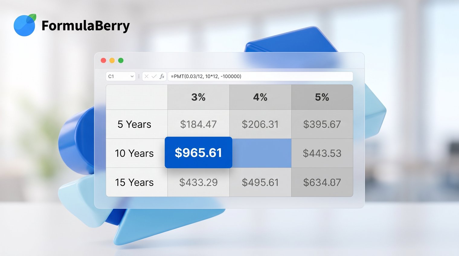
A single payment calculation answers one question. A small scenario table helps you decide what payment is affordable before you apply or sign.
Start with a base loan amount, term, and interest rate in clearly labeled cells. Then create columns for several rates or rows for several loan amounts. For example, you could compare a $225,000, $250,000, and $275,000 loan across rates of 6%, 6.5%, and 7%.
If your annual rate remains in B2 and the loan term remains in B3, a formula copied across a table might look like this:
=PMT($B$2/12,$B$3*12,-C6)
The dollar signs lock B2 and B3 in place when you copy the formula. C6 remains relative so it can change to each loan amount in your table. Without absolute references, Excel may shift your rate or term references into unrelated cells as you copy.
Round only for display whenever possible. Keep the full PMT result in the formula, then format the cell to show two decimal places. Rounding the payment inside every calculation can create small balance differences later in an amortization schedule.
Create an Amortization Schedule After You Calculate PMT
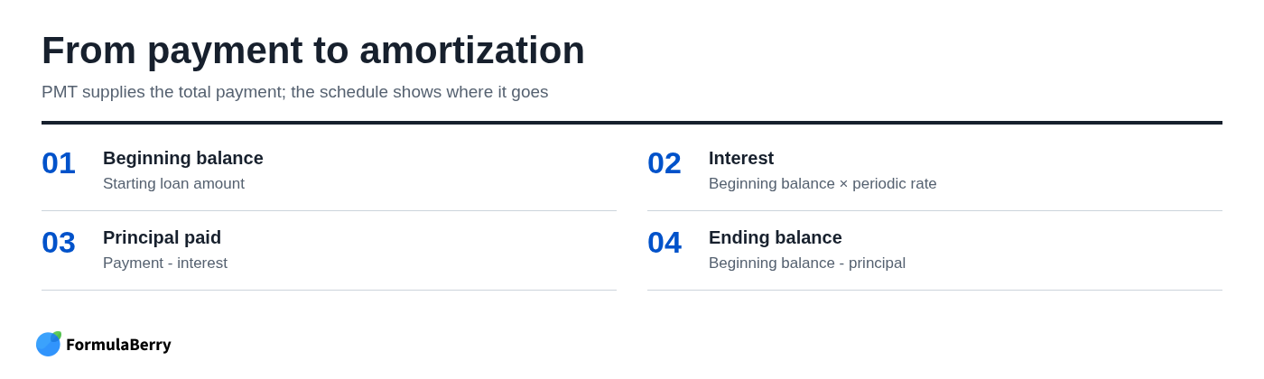
PMT tells you the total periodic payment. An amortization schedule shows how much of each payment goes to interest, how much reduces principal, and how the remaining balance changes over time.
Create columns for payment number, beginning balance, payment, interest, principal paid, and ending balance. For the first row, use the original loan amount as the beginning balance. Then calculate:
- Interest: Beginning balance multiplied by the periodic interest rate.
- Principal paid: Total payment minus interest.
- Ending balance: Beginning balance minus principal paid.
For a monthly loan, if your payment is in B6 and your annual rate is in B2, the interest formula for a row with beginning balance in C10 could be:
=C10*($B$2/12)
If the payment is stored as a positive number in B6, principal paid could be:
=$B$6-D10
Then calculate ending balance with:
=C10-E10
In the next row, set beginning balance equal to the prior row's ending balance. Copy the formulas down for the full number of payments. Early payments will be interest-heavy; later payments will direct more money to principal as the balance falls.
Check the Final Balance
After the final payment, the ending balance should be at or very near zero. A tiny residual can happen when you round payment amounts or intermediate values too early.
Use the unrounded PMT output in your amortization formulas and apply currency formatting only for display. If your final balance is still materially different from zero, recheck the rate frequency, number of periods, and sign used for the payment and principal columns.
Fix Common PMT Formula Errors
Most PMT problems come from input formatting or inconsistent time periods rather than a complicated Excel issue.
- #NUM!: Check that the rate and number of periods are valid. A negative or zero number of periods, for example, will not produce a usable loan payment.
- #VALUE!: One or more cells may contain text instead of a number. Re-enter the rate, years, or amount as numeric values and apply formatting afterward.
- Unexpected negative payment: Excel is following cash-flow sign rules. Use -B4 for the loan amount if you want the payment displayed as positive.
- Payment looks unrealistically low or high: Confirm that you divided an annual rate by 12 and multiplied years by 12 for a monthly payment.
Another frequent error is entering 6.5 when you mean 6.5%. Excel treats 6.5 as 650%, which produces a wildly incorrect result. Enter 6.5% or 0.065 instead.
Before relying on an estimate, compare the loan amount, rate basis, term, payment frequency, and first-payment timing against the lender's disclosure. If you need to calculate an implied interest rate from known loan details, see this RATE formula guide. A PMT formula is excellent for planning, but it cannot account for terms you did not enter.
Use PMT with Optional Future Value and Payment Timing
Most readers can skip the optional arguments, but they matter in a few cases.
Use fv when the loan should have a balance remaining after the last scheduled payment. For example, a balloon-loan arrangement may require regular payments while leaving a final balance due. In that case, include the desired ending balance as the fourth argument. For broader savings and loan balance calculations, see this FV Formula in Excel guide.
The type argument controls when payment occurs:
- 0: Payment at the end of the period. This is the default and the right choice for most loans.
- 1: Payment at the beginning of the period. Use this only when the contract specifically requires advance payments.
For example, a payment due at the beginning of every month could use:
=PMT(B2/12,B3*12,-B4,0,1)
Because each payment arrives earlier, a beginning-of-period payment is generally slightly lower than an otherwise identical end-of-period payment.
Calculate a Reliable Payment Before You Commit
A reliable payment formula follows three rules: match the rate to the payment frequency, match the number of periods to that same frequency, and use a negative principal value when you want Excel to return a positive payment amount.
For a standard monthly loan, =PMT(annual rate/12, years*12, -loan amount) is the simple payment formula Excel users need most often. Then build an amortization schedule to confirm how the payment divides between interest and principal over the life of the loan.
If you need help turning a specific loan scenario into an Excel or Google Sheets formula, FormulaBerry can generate, explain, or help correct the formula from a plain-language request.