
The hardest part of finding a loan's interest rate in Excel is not typing the formula. It is getting the timing, payment signs, and annual conversion right. A single mismatch can turn a reasonable monthly rate into a misleading annual percentage or a frustrating #NUM! error.
Excel's RATE function solves that problem when you know the loan amount, payment, and repayment term but need to find the implied interest rate. Here is how to set it up, calculate the result, annualize it correctly, and troubleshoot common failures.
What the Excel RATE Function Calculates
The Excel RATE function calculates the periodic interest rate implied by a series of equal payments. In other words, it solves for the unknown rate when you already know the number of payments, the payment amount, and the starting loan balance or investment amount.
RATE does not calculate a loan payment or tell you how much you can borrow. Use PMT when the payment is unknown, and use PV when the starting principal is unknown. RATE is specifically the formula for finding the rate.
The period matters. If your model uses monthly payments, RATE returns a monthly interest rate. If it uses annual payments, RATE returns an annual rate. Excel does not automatically convert the result based on how you label a cell.
Set Up Your Loan Inputs Before Writing RATE
Start with a simple, labeled worksheet. Keeping each input in its own cell makes the formula easier to audit and prevents hard-coded numbers from becoming a problem later.
| Cell | Label | Example value |
|---|---|---|
| B2 | Loan amount | 20000 |
| B3 | Monthly payment | 400 |
| B4 | Loan term in months | 60 |
| B5 | Payments per year | 12 |
| B6 | Balloon balance, if any | 0 |
Use the same time unit everywhere. For a five-year loan with monthly payments, use 60 periods, not 5. For annual payments over five years, use 5 periods. This is the source of many incorrect Excel RATE calculations for annual figures.
Also follow Excel's cash-flow sign convention: money received and money paid must have opposite signs. If the borrower receives $20,000, enter the present value as positive 20000 and the monthly payment as negative -400. You can reverse both signs, but do not make them both positive or both negative.

Understand the RATE Formula Syntax
The full syntax is:
=RATE(nper, pmt, pv, [fv], [type], [guess])
For a standard loan that is fully paid off through equal end-of-month payments, the plain-English version is: "Find the monthly interest rate that turns this loan balance into these payments over this many months."
RATE belongs to the same family of financial functions as PV, PMT, and FV, but each solves for a different unknown. RATE is the right choice only when the unknown is the interest rate.
Required Arguments: NPER, PMT, and PV
NPER is the total number of payment periods. A five-year loan paid monthly has 5 x 12, or 60 periods.
PMT is the amount paid every period. For the borrower in a standard loan model, enter it as a negative value.
PV means present value: the amount borrowed or the value today. In a borrower-focused loan worksheet, this is usually a positive number.
For example, a $20,000 loan repaid with 60 monthly payments of $400 uses 60 for NPER, -400 for PMT, and 20000 for PV.
Optional Arguments: FV, Type, and Guess
FV is the future value or remaining balance after the final listed payment. Leave it blank, or use 0, for a fully amortizing loan. Use it for a balloon loan or an investment with a target ending balance.
Type controls payment timing. Use 0, or omit the argument, when payments are made at the end of each period. Use 1 when payments are made at the beginning of each period.
Guess gives Excel a starting point for its calculation. Most simple loans do not need one. If you do use a guess in a monthly model, enter a monthly rate, not an annual rate. For example, 0.01 means 1% per month, not 1% per year.
Calculate the Monthly Interest Rate for a Loan
Suppose you borrow $20,000 and repay it with 60 monthly payments of $400. Enter this formula:
=RATE(60,-400,20000)
The result is approximately 0.006183, or about 0.6183% per month. Format the result cell as Percentage if you want Excel to display it as 0.62% rather than a decimal.
With the worksheet layout above, use cell references instead of typing values directly:
=RATE(B4,-B3,B2)
If B3 already contains -400 rather than 400, do not add the minus sign again. Use =RATE(B4,B3,B2). The goal is opposite signs between the loan amount and payment, not a particular visual format in every cell.
Convert the Periodic Result Into an Annual Rate
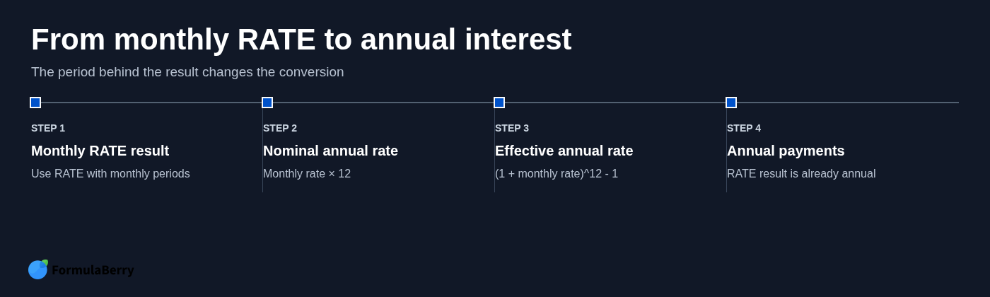
A monthly RATE result is not an annual rate. This distinction is essential when comparing your calculation with a quoted loan rate, APR, or investment return.
For a nominal annual rate, multiply the monthly rate by 12:
=RATE(B4,-B3,B2)*12
Using the example monthly rate of about 0.6183%, the nominal annual rate is about 7.42%.
If interest compounds monthly, calculate the effective annual rate instead:
=(1+RATE(B4,-B3,B2))^12-1
This gives approximately 7.68% in the example. It is higher because each month's interest becomes part of the balance used to calculate later interest.
Do not treat nominal annual rate, effective annual rate, and advertised APR as interchangeable. An APR may reflect a lender's disclosure rules and may account for charges or use conventions that differ from a simple monthly-rate conversion.
Use RATE for Other Payment Schedules and Remaining Balances
RATE works with weekly, quarterly, monthly, or annual payments as long as NPER and PMT use the same schedule. The returned result is always the rate for that schedule.
- For weekly payments, enter the total number of weeks and interpret the answer as a weekly rate.
- For quarterly payments, enter the number of quarters and interpret the answer as a quarterly rate.
- For annual payments, enter years as NPER. The returned rate is already annual, so do not multiply it by 12.
This is why an Excel model using monthly RATE periods needs annualization, while an annual payment model generally does not. The function does not know whether an input period represents a month, quarter, or year; it only sees a sequence of equal periods.
For a balloon loan, include the balance still owed at the end. Assume a $20,000 loan has 60 payments of $300 and a final balloon balance of $5,000. From the borrower's perspective, both the regular payments and final balance are cash paid out:
=RATE(60,-300,20000,-5000)
A common mistake is entering the balloon balance as positive while also using a positive loan amount. That breaks the cash-flow relationship and can produce an error or an implausible result.
When Payments Are Made at the Beginning of Each Period
Most loans use end-of-period payments, which is Excel's default type of 0. But some arrangements require payment at the beginning of the period. Examples include certain leases, rent-like agreements, and regular deposits made on the first day of each month.
Add 1 as the Type argument for beginning-of-period payments:
=RATE(60,-400,20000,0,1)
Payment timing changes the answer because each payment has one extra period to affect the balance. Do not use type=1 simply because the first payment is due soon; use it only when every scheduled payment is at the beginning of its period.
Fix #NUM! and Other RATE Formula Errors
RATE uses an iterative calculation to find a solution. Unlike a simple addition formula, Excel may need several attempts to converge on a rate. That is why errors often point to a model issue rather than a typo in the function name.
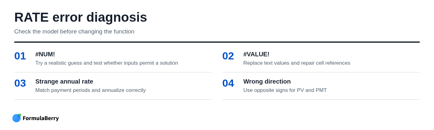
#NUM! commonly means Excel could not find a workable rate. The inputs may be incompatible, the payment may not support a payoff under the stated terms, or Excel may need a more realistic starting guess.
#VALUE! usually means at least one argument contains text, an invalid cell reference, or a value Excel cannot interpret as a number. Check cells that look numeric but may contain imported currency symbols, spaces, or text-formatted numbers.
An answer can also be technically valid but financially wrong. Extremely high or negative results often come from mixing months and years, using the same sign for PV and PMT, or annualizing a rate that was already based on annual periods.
Use a Better Guess When RATE Cannot Converge
Start by adding a realistic Guess value as the sixth argument. For a likely monthly rate, try 0.01:
=RATE(60,-400,20000,0,0,0.01)
For a model built with annual payment periods, 0.1 is a reasonable starting point when you expect something near 10% annually:
=RATE(5,-5000,20000,0,0,0.1)
Guess is only a starting point for Excel's iterative process. It is not a rate you are telling Excel to accept. If several reasonable guesses fail, stop changing guesses and check whether the payment, timing, and final balance can actually describe a valid financial arrangement.
Check Signs and Periods Before Changing the Formula
Use this order when troubleshooting a RATE formula:
- Confirm PV and PMT have opposite signs.
- Make sure the number of periods matches the payment frequency.
- Verify the payment amount can reasonably amortize the balance over the stated term.
- Check whether there is a remaining balance that belongs in FV.
- Confirm whether payments occur at the beginning or end of the period.
Pay particular attention to the payment amount. If it is lower than the periodic interest that would accrue at the rate you expect, there may be no conventional payoff rate for the stated term. In that case, RATE is not malfunctioning; the assumptions need to change.
Validate the Result With PMT and a Loan Schedule
Do not stop once RATE returns a percentage. A quick reverse check with PMT confirms that the calculated periodic rate reproduces the payment you entered.
If the calculated monthly rate is in B7, use:
=PMT(B7,B4,B2)
For the $20,000, 60-month example, PMT should return approximately -400. Small differences can occur from rounding if you display only a few decimal places in the rate cell, so keep the full stored precision for calculations.
A basic amortization schedule provides another useful check. Create columns for payment number, opening balance, payment, interest, principal repaid, and closing balance. If the ending balance does not reach zero when FV is zero, revisit the rate, payment timing, and sign convention.
For a balloon loan, validate the ending balance with FV. The final projected balance should match the balloon amount you included in the RATE formula.
Know When RATE Is Not the Right Financial Function
RATE is powerful, but it is not the right financial function for every spreadsheet finance problem.
- Use PMT when you know the rate, term, and principal but need the periodic payment.
- Use PV when you know the rate, payment, and term but need the amount that can be borrowed or invested today.
- Use FV when you need the ending balance after regular payments or deposits.
- Use IRR when cash flows vary from period to period rather than staying equal.
For example, RATE fits a fixed-payment loan. It is not the best fit for an investment with irregular deposits, skipped payments, or a changing payment amount. Trying to force irregular cash flows into RATE can produce a number, but not necessarily a useful answer.
Get a Reliable RATE Result Every Time
For a dependable RATE formula Excel calculation, choose the payment period first, use that same period for NPER and PMT, and enter cash received and cash paid with opposite signs. Solve the periodic rate before converting it to an annual figure, then validate the result with PMT or an amortization schedule.
If your worksheet has unusual payment timing, a balloon balance, or a stubborn error, FormulaBerry can help generate, explain, or correct a RATE formula from the specific inputs in your Excel or Google Sheets model.