
A column of test scores can tell you who passed, but it does not tell you what the class performance looks like. For that, you need grouped counts: how many scores fall in each range, whether results cluster in the middle, and whether any values sit outside the expected scale.
Google Sheets can build that summary with one formula. In this example, 30 raw scores become a refreshable frequency distribution table and an optional chart that updates whenever the source data changes.
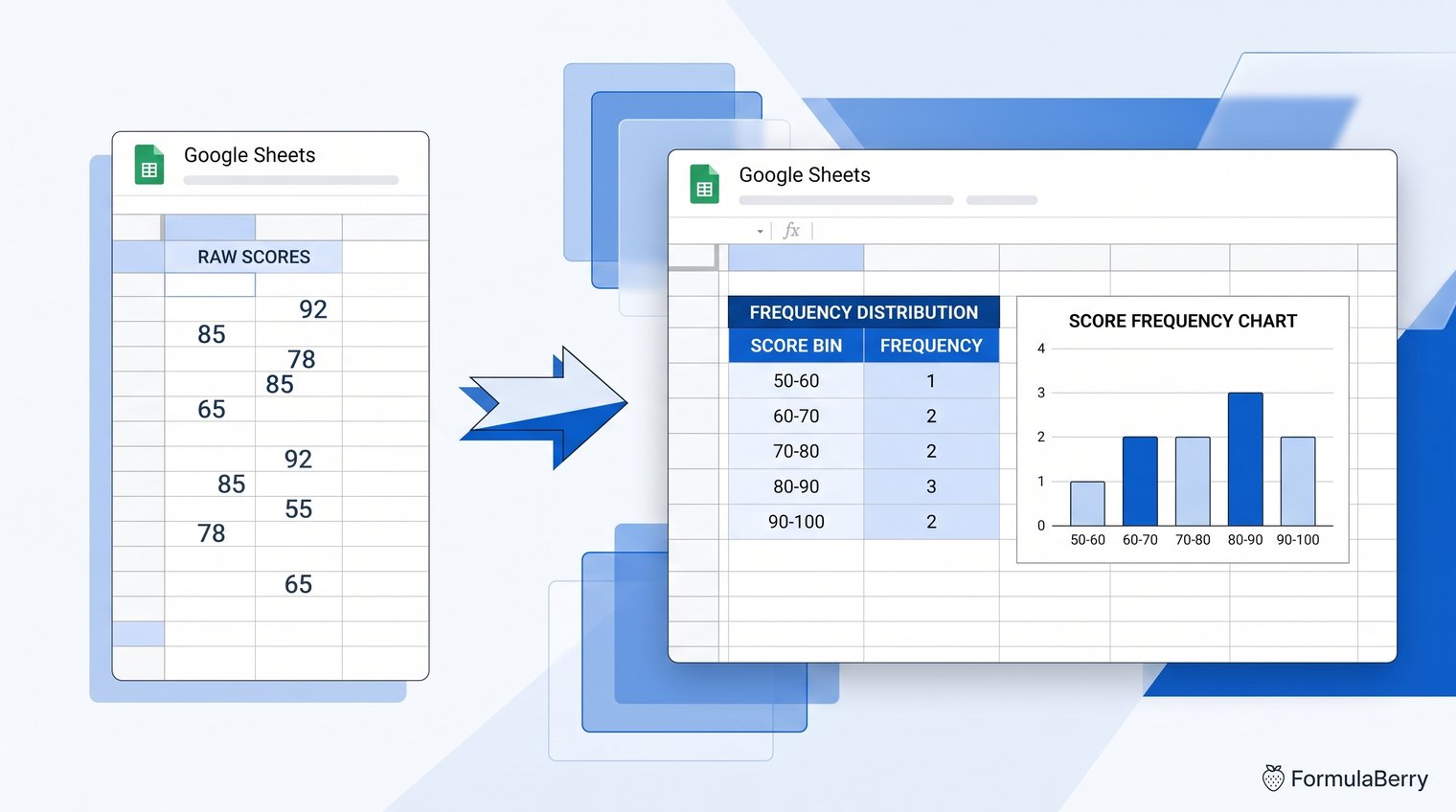
The finished result: a refreshable frequency distribution from raw scores
Suppose a teacher, tutor, or training manager has 30 test scores in column A. Reading them one at a time is slow, especially when the real question is whether the group is concentrated around passing grades or spread across the entire range.
The finished sheet has three useful pieces: the raw scores, a numeric bin column used by the formula, and readable score-range labels for people viewing the report. The frequency counts recalculate automatically when a score is added or changed.
What the FREQUENCY formula does in Google Sheets
The FREQUENCY formula counts numeric values into intervals defined by bin limits. Its basic pattern is:
=FREQUENCY(data_range, bins_range)
The formula returns an array of counts, not a single number. If you provide six bin limits, Google Sheets returns seven results: one count for each bin and one extra count for values greater than the final bin.
That final result is easy to miss, but it matters. A frequency distribution should account for every numeric observation, including unexpected values such as a score above 100.
FREQUENCY is also different from a simple unique-value count. A unique-value count might tell you that three people scored 72 and two scored 84. A frequency distribution answers the broader question: how many people scored from 70 to 79, or from 80 to 89?
Case setup: turn 30 raw test scores into score ranges
For this illustrative example, place 30 test scores in cells A2:A31. The list can be in any order. It might include values such as 43, 58, 60, 72, 88, 94, and 103 alongside the rest of the class results.
The goal is to create this score distribution:
| Score range | Upper bin limit | What it counts |
|---|---|---|
| 0-49 | 49 | Scores up to and including 49 |
| 50-59 | 59 | Scores from 50 through 59 |
| 60-69 | 69 | Scores from 60 through 69 |
| 70-79 | 79 | Scores from 70 through 79 |
| 80-89 | 89 | Scores from 80 through 89 |
| 90-100 | 100 | Scores from 90 through 100 |
| >100 | Overflow | Scores above 100 |
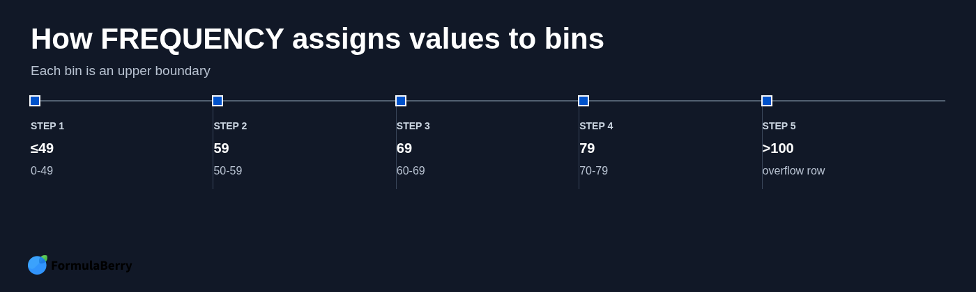
Enter the upper limits 49, 59, 69, 79, 89, and 100 in C2:C7. They must be sorted in ascending order. FREQUENCY reads each number as the top boundary of a range, not as a category label.
In plain language, the desired output is: count how many of the 30 scores fall into each score band, and flag anything above 100 instead of silently losing it.
Choose bins that match the question you need to answer
Bin width changes the story your data tells. Ten-point score bands are usually practical for test results because they align with familiar grade ranges and make a compact report.
Narrower bins reveal more variation. If you were reviewing the effectiveness of a short quiz, five-point intervals could show whether scores are tightly clustered. Broader bins summarize faster, but they can hide meaningful differences between results.
The boundary rule is the detail that causes most errors. With bin limits of 49 and 59, the first bin includes values less than or equal to 49, while the next bin includes values greater than 49 and less than or equal to 59. A score of 59 belongs in 50-59, not in the next range.
Build the frequency table with the FREQUENCY formula
With raw scores in A2:A31 and bin limits in C2:C7, click the first output cell, such as D2, and enter:
=FREQUENCY(A2:A31,C2:C7)
The first argument, A2:A31, is the data range containing the scores. The second argument, C2:C7, is the ordered list of numeric upper limits.
Modern Google Sheets spills the results downward automatically. Because there are six bins, the formula needs seven empty output cells: D2:D8. Do not type counts into those cells or copy the formula down one row at a time. One FREQUENCY formula creates the complete array.
For a representative set of 30 scores, the result could look like this:
| Bin limit | Frequency |
|---|---|
| 49 | 3 |
| 59 | 4 |
| 69 | 6 |
| 79 | 8 |
| 89 | 5 |
| 100 | 3 |
| >100 | 1 |
Those example counts total 30, which is exactly what a complete distribution should do when all 30 source cells contain numeric scores.
Formula pattern you can reuse
The reusable frequency formula in Google Sheets is:
=FREQUENCY(data_range, bins_range)
For example, a small business tracking order values might use a data range of invoice totals and bin limits of 100, 250, 500, and 1000. The formula itself does not change; only the data and the boundaries do.
If you plan to copy a reporting layout across columns or tabs, absolute references can help. For example:
=FREQUENCY($A$2:$A$31,$C$2:$C$7)
For a single table, standard references are easier to read and work just as well.
Read the extra overflow result correctly
The last returned value does not belong to the final bin. It counts values greater than the highest bin limit.
In this score example, the count beside 100 covers scores from 90 through 100. The next result counts only scores above 100. Label that row clearly as >100 so a reader does not mistake it for another 90-100 count.
If scores should never exceed 100, an overflow count greater than zero is useful evidence of a data-entry problem, a different grading scale, or an incorrect bin plan. You can hide the row only after checking that it is zero and deciding it is not needed in the final report.
Make the result readable with interval labels
Raw bin limits are ideal for the formula but not for the person reading the report. A stakeholder seeing 49, 59, 69, and 79 may understand the pattern, but labels remove the need for interpretation.
Create a companion label column in B2:B8:
| Cell | Label |
|---|---|
| B2 | 0-49 |
| B3 | 50-59 |
| B4 | 60-69 |
| B5 | 70-79 |
| B6 | 80-89 |
| B7 | 90-100 |
| B8 | >100 |
Keep the numeric bin limits in column C for FREQUENCY, keep the counts in column D, and use the labels in column B for reports and charts. This separation is simple, but it prevents a common mistake: replacing numeric bins with text labels and then wondering why the formula no longer works.
Before and after: verify the counts against the raw data
A frequency table is only useful if it reflects the source records. Before sharing it, spot-check a few values and reconcile the total.
In the raw list, a score of 49 belongs in the 0-49 row because the first bin includes values less than or equal to 49. A score of 60 belongs in the 60-69 row because it is greater than the prior boundary of 59 and less than or equal to 69.
If the source list includes 103, it should appear only in the >100 overflow row. It should not inflate the 90-100 count. That distinction is precisely why the overflow output needs to stay visible while you validate the table.
Finally, add the frequency results together. In this representative case, the seven counts total 30. You can use the Google Sheets SUM formula to check that total. If your result is lower than the number of records you expected, check whether some source cells contain text, blanks, error values, or values outside a range that was not captured properly.
Create a frequency chart from the completed table
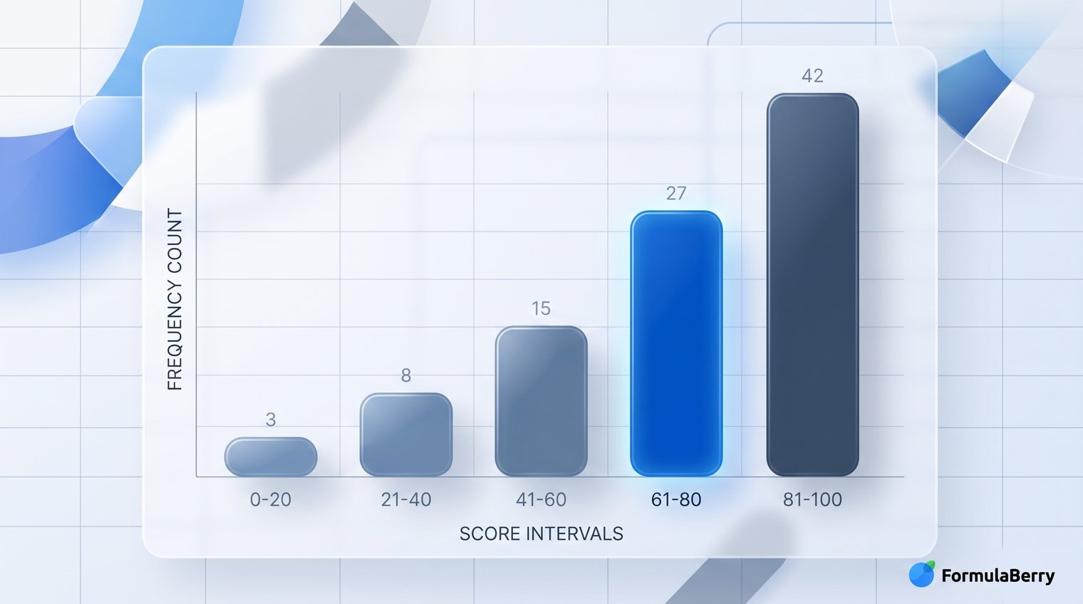
Once the frequency distribution table is correct, turning it into a Google Sheets frequency chart is straightforward. Select the interval labels and frequency counts, such as B2:B8 and D2:D8, then choose Insert > Chart.
A column chart is usually the clearest choice. Keep the categories in ascending score order, with 0-49 at the left and >100 at the right. The vertical axis represents the number of scores in each interval.
This is not quite the same thing as using Google Sheets' built-in histogram option. A histogram can generate its own groupings, while this chart uses the deliberate bin plan you already defined. When the assignment, business rule, or reporting standard requires fixed ranges, charting the completed frequency table gives you more control.
Because the chart is connected to the formula output, it updates when the source scores change. Add a new score, and the relevant interval count and chart bar adjust automatically.
For a compact dashboard, you could also compare this approach with the Google Sheets SPARKLINE formula, which creates a small chart inside a cell rather than a full chart object.
When COUNTIF or a pivot table is the better choice
FREQUENCY is excellent for repeatable numeric binning, but it is not the only way to count in Google Sheets.
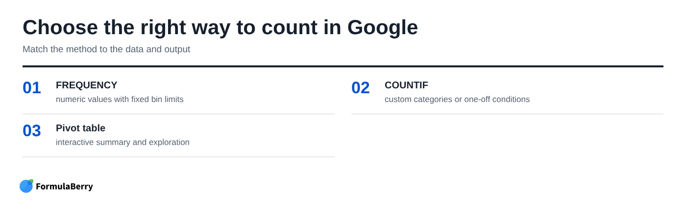
- Use FREQUENCY when you have numeric data and fixed upper boundaries, such as score ranges, spending bands, response times, or order-value brackets.
- Use COUNTIF or COUNTIFS when categories are custom, text-based, or need unrelated conditions. For example, count orders marked "Paid," "Pending," and "Overdue," or count scores above 80 for one instructor.
- Use a pivot table when you want to explore a dataset interactively, summarize several fields, or rearrange the view without building a formula-driven report.
A COUNTIFS setup can reproduce numeric ranges, but it becomes repetitive when many bands are involved. FREQUENCY keeps the ranges in one ordered bin list and returns all counts at once, which is cleaner for a stable frequency distribution table.
Common FREQUENCY formula problems and how to fix them
When FREQUENCY appears not to work, the formula is often fine. The issue is usually the bin list, the source data, or the cells below the formula.
Start with a quick diagnostic sequence: confirm that the data range contains real numbers, inspect the bin range, sort bins from smallest to largest, clear the expected spill area, and compare the sum of all frequency results with the number of numeric records.
Bins out of order are particularly misleading. A list such as 59, 49, 69 does not describe a valid ascending set of boundaries. Sort it to 49, 59, 69 before trusting any output.
Also watch for numbers stored as text. A score that looks like 78 may not be counted if it was imported with a leading apostrophe, hidden spaces, or inconsistent formatting. Converting those cells to numeric values often resolves a total that seems too low.
The output does not spill into enough rows
FREQUENCY always returns one more result than the number of bins. Six bin limits require seven output rows.
If Google Sheets cannot expand the formula, inspect the cells beneath it. A typed value, another formula, or even a stray note in the spill range can block the array. Clear the occupied cells in the output area, then keep the FREQUENCY formula only in the top cell. Do not copy it downward.
Counts look wrong at bin boundaries
Remember that each listed bin is an inclusive upper boundary. The lower boundary comes from the prior bin.
With bins of 59 and 69, a score of 60 belongs in 60-69 because it is greater than 59 and less than or equal to 69. A score of 69 also belongs there. A score of 70 moves to the next row.
Apply the same pattern to your own data
The test-score example is easy to transfer to budgets, sales values, delivery times, survey ratings, or any other numeric list. The reliable workflow is the same:
- Identify the numeric data you want to summarize.
- Choose bin limits that answer a useful business or reporting question.
- Enter the limits in ascending order.
- Use =FREQUENCY(data_range, bins_range) once in the first output cell.
- Add readable interval labels alongside the numeric bins.
- Keep and check the overflow result.
- Verify that the counts total the numeric observations, then chart the results if a visual summary helps.
If you are adapting the formula to an unfamiliar layout, the Google Sheets Formula Generator can turn a plain-language request into a formula or explain an existing one before you place it in the sheet. You can also visit FormulaBerry for more spreadsheet guidance.
The two details that make a frequency distribution reliable are simple: bins must be ordered upper limits, and the final overflow row must be accounted for. Get those right, and your raw scores become a summary people can actually use.