

Date formulas in Google Sheets are simple until a deadline lands at month-end, an imported date swaps the day and month, or a result turns into a five-digit number. Most date problems are not really formula problems. They start with data that looks like a date but is actually text, or with a display format that hides what Sheets is calculating.
This guide covers how to create dates, calculate deadlines and workdays, extract reporting periods, format dates as dd/MM/yyyy, and diagnose the errors that make otherwise sensible formulas fail.
How Google Sheets stores dates (and why formulas sometimes fail)
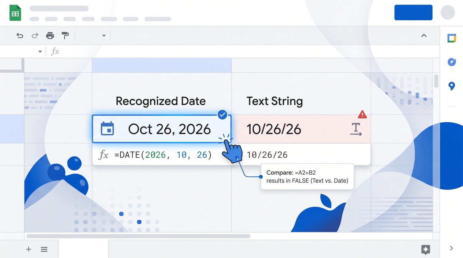
Google Sheets stores a real date as a serial number. The displayed date is simply formatting applied to that number. For example, a date can display as 12/11/2026, 12 Nov 2026, or Thursday, 12 November without changing the underlying value.
Times use the decimal portion of the same serial value. A whole number represents a date, while a fraction represents a time during that day. This is why subtracting one date-time value from another can return a decimal number of days.
That distinction matters because Google Sheets can only calculate reliably with real date values. The common causes of broken date formulas are:
- Dates stored as text: A value such as "12/11/2026" may look right but cannot always be added, subtracted, or compared.
- Locale mismatches: One spreadsheet may interpret 04/05/2026 as 4 May, while another treats it as 5 April.
- Ambiguous entry formats: A typed slash-separated date is risky when both the day and month are 12 or lower.
- Formatting confusion: A valid calculation may return a number because the result cell is formatted as General rather than Date.
Keep three separate jobs in mind: entering or creating a valid date, calculating with that date, and formatting how it appears. Formatting is cosmetic. It does not fix a text value or change how Sheets interpreted a date when it was entered.
Quick start: the date formulas most people need
| Task | Formula | What it returns |
|---|---|---|
| Today's date | =TODAY() | The current date, updated when the sheet recalculates. |
| Add seven days | =A2+7 | A date seven calendar days after A2. |
| Days between dates | =A2-B2 | The difference in days, including a negative result if A2 is earlier. |
| Create a fixed date | =DATE(2026,11,12) | 12 November 2026 as a real date value. |
| End of the month | =EOMONTH(A2,0) | The final day of A2's month. |
| Extract the year | =YEAR(A2) | The four-digit year from A2. |
These formulas cover a surprising amount of everyday work. The sections below explain when simple arithmetic is enough, when you need calendar-aware functions such as EDATE or EOMONTH, and how to avoid text and locale traps.
Create dates with DATE, TODAY, NOW, and DATEVALUE
The safest date formulas produce real date values from the start. That is better than joining text fragments such as a year, month, and day with slashes and hoping Sheets reads the result correctly.
Build reliable dates with DATE(year, month, day)
The DATE function creates a date from separate numeric inputs:
=DATE(2026,11,12)
This returns 12 November 2026. DATE is especially useful when the year, month, and day are stored in separate columns, such as A2 for year, B2 for month, and C2 for day:
=DATE(A2,B2,C2)
Do not replace this with =A2&"/"&B2&"/"&C2. Concatenation creates text, and whether that text converts to a date may depend on the spreadsheet locale.
DATE also handles month overflow. For example, =DATE(2026,13,1) returns 1 January 2027. That can be useful in formulas that intentionally roll forward by months, but it can also conceal bad source data. If month 13 was a mistake, validate the input rather than relying on DATE to silently normalize it.
Insert today's date or the current date and time
Use =TODAY() when you need today's date. Use =NOW() when you need both the current date and time. Both formulas are volatile, meaning they recalculate as the spreadsheet updates. They are useful for live reporting, overdue flags, and current-period calculations, but they are not permanent timestamps.
If you need a fixed date that will not change tomorrow, enter it manually with the keyboard shortcut Ctrl+; on Windows or ChromeOS, or Cmd+; on Mac. On a phone or tablet, use the date picker if available, or enter a clear date directly into the cell and verify the displayed value.
A common mistake is using TODAY() to record when an order was received or a task was completed. It will display the correct date initially, then change. For an audit trail, use a static entry instead.
Convert date-looking text with DATEVALUE
DATEVALUE converts recognizable date text into a date serial number. If A2 contains text such as 12 November 2026, use:
=DATEVALUE(A2)
Then apply a date format to the result cell. DATEVALUE is useful for unambiguous text, particularly dates with written month names. It is risky with values such as 04/05/2026 because the function follows your sheet's locale rules.
When source data is split into separate year, month, and day columns, use DATE instead. It is more explicit, more portable, and far less likely to turn 4 May into 5 April.
Add and subtract days, weeks, months, and years
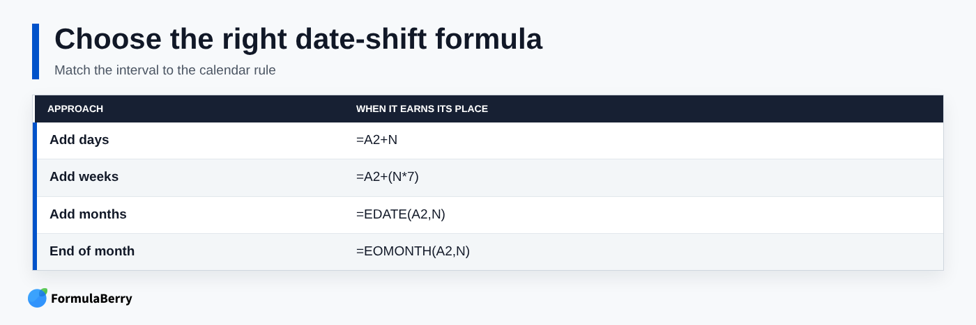
Date arithmetic drives practical spreadsheet work: delivery deadlines, follow-up dates, subscription renewals, billing cycles, and aging reports. The key is matching the formula to the rule. Adding 30 days and adding one calendar month are not the same instruction.
Add or subtract days and weeks
Because dates are numbers, add or subtract whole numbers for calendar days:
- =A2+14 adds 14 days.
- =A2-7 returns the date seven days earlier.
- =A2+(B2*7) adds the number of weeks specified in B2.
If the result displays as a number, the formula is still likely correct. Format the output cell as a date. Simple arithmetic counts every day, including weekends and holidays, which is exactly right for calendar-day policies.
Shift calendar months with EDATE
Use EDATE when the requirement is stated in calendar months:
- =EDATE(A2,3) adds three months.
- =EDATE(A2,-1) subtracts one month.
EDATE is preferable to adding 30 or 31 days. A 30-day shift from 31 January is not the same as one month later, and the difference becomes important in contracts, recurring invoices, and renewal dates.
For month-end dates, EDATE follows the calendar as closely as possible. A date such as 31 January shifted one month forward lands at the last valid day in February. That is normally the behavior people want for recurring monthly schedules.
Move years with EDATE and EOMONTH
To move to the same calendar month next year, use:
=EDATE(A2,12)
This is often cleaner than trying to rebuild a date with YEAR, MONTH, and DAY. Leap-day records deserve special attention: a date on 29 February cannot map to 29 February in a non-leap year, so Sheets adjusts to a valid date.
EOMONTH returns the final day of a month:
- =EOMONTH(A2,0) returns the end of A2's month.
- =EOMONTH(A2,1) returns the end of next month.
Use EOMONTH for month-end billing, closing reports, and periods that must end on the actual final calendar day rather than after an arbitrary number of days. For more examples, see this Google Sheets End of Month Formula guide.
Calculate days, workdays, and date differences
Knowing that two dates are different is not enough for a project schedule or aging report. You need to know whether the difference is calendar days, complete months, or working days under your organization's weekend and holiday rules.
Find the number of days between two dates
The most direct formula is:
=B2-A2
If A2 is the start date and B2 is the end date, the result is the number of days between them. It excludes the start date itself. For example, 1 June to 2 June returns 1.
You can also use =DATEDIF(A2,B2,"D"), which returns the same whole-day interval. Simple subtraction is usually easier to audit. DATEDIF becomes more useful when you need completed months or years.
A negative result means the dates are reversed. Use =ABS(B2-A2) only when direction truly does not matter, such as measuring the gap between two events. Do not use ABS to hide a scheduling error in a due-date report.
Count complete months and years with DATEDIF
DATEDIF counts fully completed intervals:
- =DATEDIF(A2,B2,"M") returns complete months.
- =DATEDIF(A2,B2,"Y") returns complete years.
Suppose a customer subscription began on 15 January 2025 and you check it on 14 January 2026. =DATEDIF(start,end,"Y") returns 0 because a full year has not yet been completed. On 15 January 2026, it returns 1.
DATEDIF expects the end date to be later than the start date. Reversed inputs can produce an error, so validate date order before using it in a large report.
Calculate working days and due dates
For business-day calculations, use NETWORKDAYS and WORKDAY instead of manually subtracting weekends.
- =NETWORKDAYS(A2,B2) counts working days from start to end, including both dates when they are workdays.
- =NETWORKDAYS.INTL(A2,B2,weekend_pattern) supports custom weekend arrangements.
- =WORKDAY(A2,5) returns the date five working days after A2.
Add a holiday range when needed. For example, =WORKDAY(A2,5,$H$2:$H$12) excludes dates listed in H2:H12. Those holiday cells must contain genuine date values, not text that merely resembles dates.
NETWORKDAYS is inclusive, while ordinary subtraction is not. That difference explains many "off by one" results. Decide whether your policy counts the request date, due date, or both before building the formula.
Extract date parts for grouping, labels, and reports
A source date should usually remain intact. Extract separate parts into helper columns when you need to group transactions by month, build labels, or apply reporting logic.
Extract year, month, day, and weekday
These functions return numbers:
- =YEAR(A2) returns the year.
- =MONTH(A2) returns 1 through 12.
- =DAY(A2) returns the day of the month.
- =WEEKDAY(A2,2) returns 1 for Monday through 7 for Sunday.
The second argument in WEEKDAY controls the numbering system. Using 2 is generally the most practical choice for workweek logic because Monday becomes 1 and Friday becomes 5. Without it, the default system begins with Sunday.
Create readable month, weekday, and quarter labels
Use TEXT when you need a readable label:
- =TEXT(A2,"mmmm") returns a full month name, such as November.
- =TEXT(A2,"ddd") returns an abbreviated weekday, such as Thu.
- ="Q"&ROUNDUP(MONTH(A2)/3,0) returns a quarter label, such as Q4.
Text labels are useful in dashboards and presentation tables, but they do not sort chronologically by themselves. A column of January, February, and March can sort alphabetically instead. Keep the original date, a numeric month, or a sortable year-month key alongside the label.
Get the start or end of a reporting period
For the first day of a month, use:
=EOMONTH(A2,-1)+1
For the end of the same month, use:
=EOMONTH(A2,0)
To calculate the Monday that begins A2's week, use:
=A2-WEEKDAY(A2,2)+1
That formula assumes a Monday-first reporting week. If your organization reports Sunday through Saturday or uses a fiscal calendar, build the convention deliberately rather than copying a formula with the wrong assumptions.
Format dates as dd/MM/yyyy without changing their value
Formatting changes how a valid date looks, not what it is. If a cell contains a real date, you can display it as dd/MM/yyyy without affecting calculations, filters, sorting, or comparisons.
Locale still matters at the moment a date is typed or imported. Formatting a cell as dd/MM/yyyy after Sheets already interpreted 04/05/2026 as April 5 does not convert it into 4 May. It only changes the display of the date Sheets has already stored.
Apply a custom date format in Google Sheets
Select the cells or entire date column, then choose Format > Number > Custom date and time. Common formats include:
- dd/MM/yyyy for 12/11/2026
- d MMM yyyy for 12 Nov 2026
- dddd, d MMMM for Thursday, 12 November
Apply the format to the full destination column before importing data or entering new records. Consistent formatting makes visual checks easier and prevents a mixture of date displays from confusing reviewers.
Convert mm/dd/yyyy to dd/mm/yyyy safely
If the cells already contain correctly recognized dates, this is only a formatting change: apply dd/MM/yyyy as described above.
If the values are text, or if they were interpreted using the wrong day/month order, do not blindly reformat the entire column. First validate a sample against a known source record. A date such as 03/04/2026 cannot tell you on its own whether it means 3 April or 4 March.
The safest reconstruction pattern is to use separate source components. If month is in A2, day is in B2, and year is in C2, use:
=DATE(C2,A2,B2)
This creates an unambiguous value, which you can then display as dd/MM/yyyy. For imported strings, parse only after you know the source convention. A display format cannot repair incorrectly interpreted historical data.
Use IF and conditional logic with dates
Date comparisons become genuinely useful when they drive a decision: mark a task overdue, identify records within an eligibility window, or show which invoices need follow-up.
Test whether a date falls between two dates
Use AND inside IF for an inclusive range test:
=IF(AND(A2>=start_date,A2<=end_date),"In range","Out of range")
This includes dates equal to the start or end boundary. Replace start_date and end_date with cell references, such as $H$1 and $H$2, if the range limits are stored in the sheet.
For larger tabular workflows, COUNTIFS is compact:
=COUNTIFS(A2,">="&$H$1,A2,"<="&$H$2)>0
It returns TRUE when A2 falls within the specified range. For more ways to count dates and other values by criteria, see this COUNTIF Formula in Google Sheets guide. As covered in the formatting section, use real date values in these comparisons, not TEXT-formatted date labels.
Flag overdue, upcoming, and missing dates
A reliable overdue label should protect blank cells:
=IF(A2="","",IF(A2<TODAY(),"Overdue","Open"))
Without the first IF check, an empty cell can be treated as an old value and incorrectly labeled overdue.
To identify items due soon, extend the logic:
=IF(A2="","",IF(A2<TODAY(),"Overdue",IF(A2<=TODAY()+7,"Due within 7 days","Open")))
Because TODAY() updates automatically, these labels change as time passes. That is desirable for an active task list, but not for a fixed historical status report.
Build a date formula that fills down automatically
Manual fill handles are useful for a short list. Formula-driven sequences and row-based logic are better when a table grows regularly and every new row should follow the same date rule.
Create a sequence of dates with SEQUENCE
To generate 30 consecutive dates beginning on 1 January 2026, use:
=SEQUENCE(30,1,DATE(2026,1,1),1)
The arguments are rows, columns, start value, and step. For weekly dates, change the final argument to 7:
=SEQUENCE(12,1,DATE(2026,1,1),7)
SEQUENCE spills results into cells below or beside the formula. Leave the intended output range empty or Sheets will return a spill error.
Generate dates from row-based inputs
For a follow-up date seven days after a trigger date in B2, use:
=IF(B2="","",B2+7)
The formula stays blank until the source date exists, then calculates the follow-up date. Fill it down a normal table, or use an array-based setup if your workflow requires one formula for an entire column.
Relative references such as B2 change as you copy a formula down. Absolute references such as $H$1 stay fixed. Use an absolute reference for one anchor date, a policy setting, or a holiday range such as $H$2:$H$12.
Troubleshoot Google Sheets date formula errors
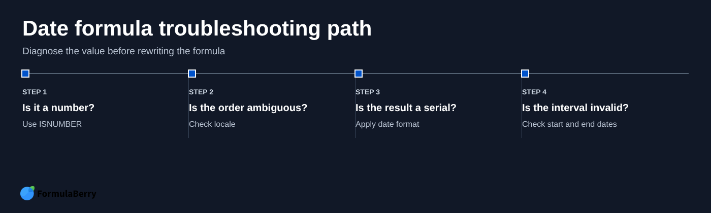
When a date formula fails, do not immediately replace it with a more complicated one. Check the input type first, then the locale, then a simple test calculation, and finally the display format. This sequence finds the real problem faster than trial and error.
Fix dates stored as text
Test whether A2 is a genuine numeric date value:
=ISNUMBER(A2)
TRUE usually means Sheets can calculate with it. However, a numeric value can still represent an unintended date or a date-time, so verify the source convention and the displayed value. You can also try:
=A2+1
If that returns an error, A2 may be text. Use DATEVALUE only for unambiguous text dates. For ambiguous imported values, rebuild them with DATE once you know which source field represents year, month, and day.
Fix locale and separator problems
Your spreadsheet locale affects both date interpretation and formula syntax. Check it under File > Settings > Locale. In some locales, formulas use semicolons instead of commas between arguments.
Avoid relying on ambiguous entries such as 04/05/2026. Use a written month, an ISO-style source format where appropriate, or the DATE function. This is especially important when a sheet is shared across regions or receives data from several systems.
Fix unexpected numbers or error values
A five-digit result is often a correctly calculated date shown in General format. Select the cell and apply a date format before assuming the formula is wrong.
#VALUE! commonly indicates invalid text where a date or number was expected. #NUM! can occur with invalid date intervals, including DATEDIF formulas where the end date is earlier than the start date. If the cell shows #####, widen the column first; the date may simply not fit in the current width.
Worked example: build a deadline tracker with calendar and business-day rules
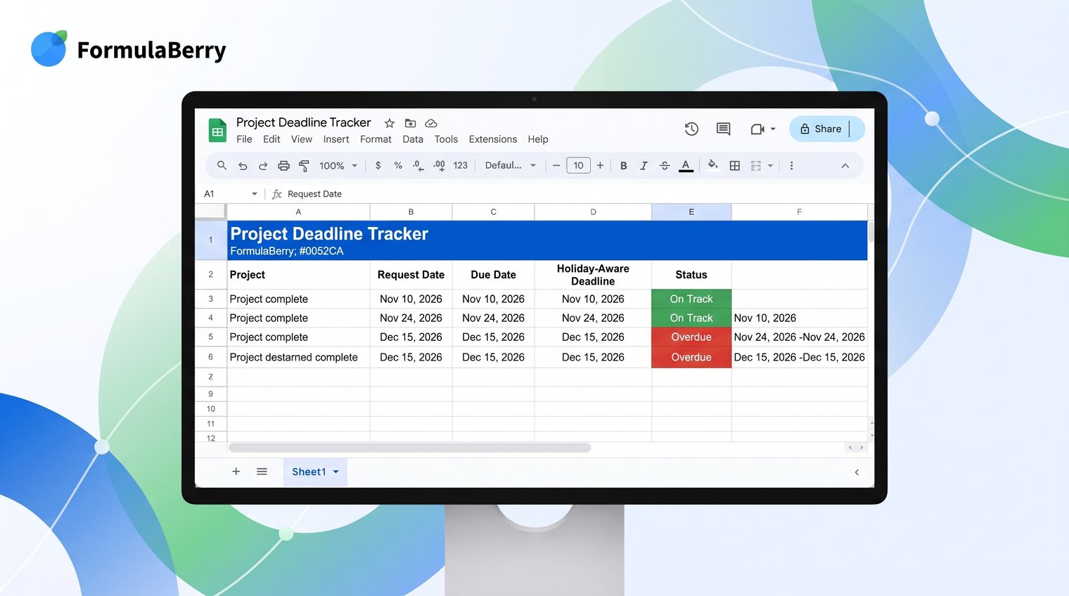
A useful deadline tracker should not force every due date into one formula. A five-calendar-day response target, a five-business-day service-level agreement, and a month-end billing rule are different policies and need different calculations.
Create a small worksheet with these columns: Request Date, SLA Type, Due Date, Days Remaining, and Status. Put company holidays in H2:H12 as real dates, and format the date columns as dd/MM/yyyy.
| Request Date | SLA Type | Due Date rule | Why it fits |
|---|---|---|---|
| 12/11/2026 | 5 calendar days | =A2+5 | Every day counts, including weekends. |
| 12/11/2026 | 5 business days | =WORKDAY(A2,5,$H$2:$H$12) | Skips weekends and listed holidays. |
| 12/11/2026 | Month-end billing | =EOMONTH(A2,0) | Uses the actual final day of the month. |
In a real tracker, you can select the correct calculation from the SLA Type column:
=IF(B2="5 calendar days",A2+5,IF(B2="5 business days",WORKDAY(A2,5,$H$2:$H$12),IF(B2="Month-end billing",EOMONTH(A2,0),"")))
For Days Remaining, subtract today from the due date:
=IF(C2="","",C2-TODAY())
Then create a readable status label:
=IF(C2="","",IF(C2<TODAY(),"Overdue",IF(C2=TODAY(),"Due today",IF(C2<=TODAY()+3,"Due soon","Open"))))
This example combines the principles from earlier sections: use real date inputs, choose calendar-aware functions for calendar rules, include holidays only in business-day logic, and keep date formatting separate from calculation. Conditional formatting can then highlight Overdue or Due soon rows without changing any formulas.
A compact Google Sheets date formula reference
| Task | Formula | Purpose and caveat |
|---|---|---|
| Create a date | =DATE(2026,11,12) | Builds a valid date from numeric parts; safer than joining text. |
| Current date | =TODAY() | Updates automatically; do not use for permanent timestamps. |
| Current date and time | =NOW() | Updates automatically and includes time. |
| Convert text | =DATEVALUE(A2) | Use only when text dates are unambiguous. |
| Add days | =A2+14 | Counts calendar days, including weekends. |
| Add weeks | =A2+(B2*7) | Multiplies the week count by seven. |
| Add months | =EDATE(A2,3) | Use for calendar months, not a 30-day approximation. |
| End of month | =EOMONTH(A2,0) | Returns the last date in A2's month. |
| Days between | =B2-A2 | Negative results indicate reversed date order. |
| Complete months | =DATEDIF(A2,B2,"M") | Counts completed months only. |
| Business days | =NETWORKDAYS(A2,B2) | Includes both endpoints when they are workdays. |
| Business-day deadline | =WORKDAY(A2,5,$H$2:$H$12) | Skips weekends and holiday dates. |
| Year | =YEAR(A2) | Returns a numeric year for grouping. |
| Month label | =TEXT(A2,"mmmm") | Returns text, so preserve a numeric sort field too. |
| Monday of the week | =A2-WEEKDAY(A2,2)+1 | Assumes Monday is the first day of the week. |
| Date in range | =AND(A2>=$H$1,A2<=$H$2) | Uses inclusive start and end boundaries. |
Use dates as values first, displays second
Reliable Google Sheets date formulas begin with valid date values. Once the input is real, use simple arithmetic for calendar days, EDATE for month shifts, EOMONTH for month-end rules, and WORKDAY or NETWORKDAYS for business schedules. Format the result only after the calculation is correct.
If you know the spreadsheet task you need but not the exact formula, FormulaBerry can help generate, explain, or correct a Google Sheets or Excel formula from a plain-English request. You can also use the Google Sheets Formula Generator for that workflow.