

A missing equals sign, one misplaced comma, or a copied reference that shifts the wrong way can turn a simple Google Sheets calculation into a frustrating error. The good news is that inserting a formula is straightforward once you understand how Sheets reads references, operators, and functions.
This guide shows how to enter formulas, add values, edit and copy them, lock references, inspect formulas, and troubleshoot the most common errors.
Quick start: Select the cell where you want the result, type =, enter an expression or function such as =A2+B2, press Enter, and verify the result in the cell or formula bar.
Start a formula in the cell where you want the result
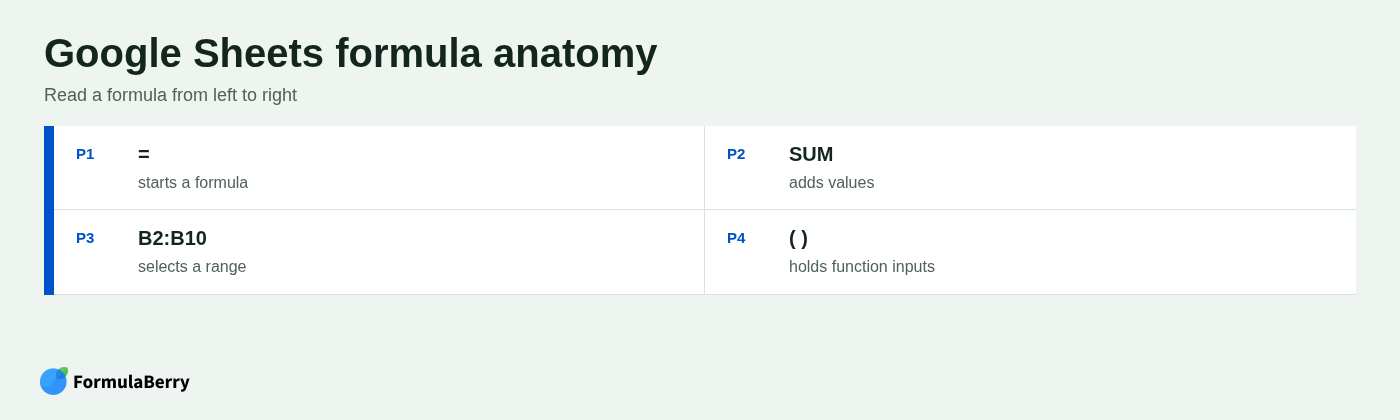
Click the cell where you want Google Sheets to display the answer, then type an equals sign (=). Every working formula starts this way. After the equals sign, add cell references, numbers, mathematical operators, or a function such as SUM.
For example, entering =A2+B2 tells Sheets to add the values currently in cells A2 and B2. You can enter the formula directly in the selected cell, type it in the formula bar above the sheet, or double-click a cell to edit its contents in place.
Press Enter to calculate the formula. By default, the cell displays the result, not the formula itself. Select the result cell and look at the formula bar whenever you need to review the underlying calculation.
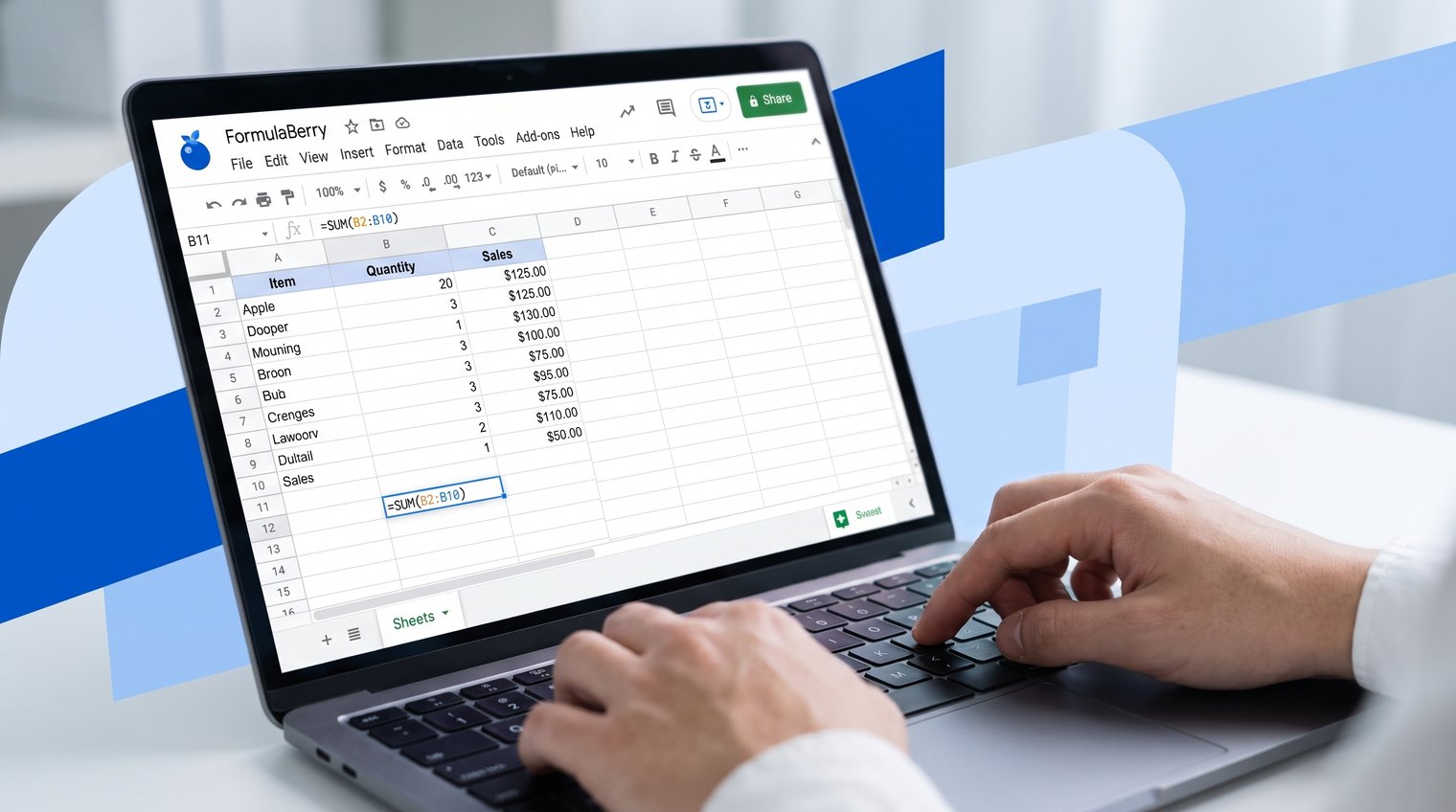
Add values with a basic Google Sheets formula
There are two sensible ways to add values in Google Sheets. Use direct addition when you are combining a small, fixed group of cells. Use SUM when you are totaling a continuous block of data.
Add two or more individual cells
To add two cells, enter:
=A2+B2
To add three individual values, extend the same pattern:
=A2+B2+C2
This is clearest when each cell has a specific meaning, such as adding a base fee, shipping cost, and tax amount from separate columns. It is less practical for a long list because each reference must be typed and maintained individually.
Add a continuous range with SUM
For a column or row of adjacent values, use SUM:
=SUM(B2:B20)
The colon means "from B2 through B20," including every cell between those two points. This is the better default for totals because new values can be included simply by adjusting the range. For more examples, see this guide to the Google Sheets SUM formula.
You can also total non-adjacent cells or ranges. For example, =SUM(B2,D2,F2) adds three separate cells, while =SUM(B2:B10,D2:D10) adds two distinct ranges.
Use cell references, operators, and functions correctly
Most Google Sheets formulas are built from a few simple parts. A cell reference points to data, an operator performs math, and a function handles a repeatable calculation. For more specialized examples, see this guide to Google Sheets custom formulas.
- Cell references: A2, B2:B10, and Sheet2!C5
- Operators: + for addition, - for subtraction, * for multiplication, and / for division
- Functions: SUM, AVERAGE, COUNTIF, and IF
Google Sheets follows the normal order of operations, so multiplication and division happen before addition and subtraction. Use parentheses when you need to control that order. For example, =A2+B2*C2 multiplies B2 by C2 first, while =(A2+B2)*C2 adds A2 and B2 before multiplying.
As you type, Sheets suggests matching functions and displays function help. Use those suggestions rather than guessing an argument order. It is a quick way to avoid syntax mistakes, especially with functions that need several inputs.
Try these common Google Sheets formula examples
You do not need to memorize hundreds of functions to work efficiently. Start with formulas that match common reporting, budget, and sales-tracking tasks.
Calculate totals and averages
=SUM(B2:B10) adds all values in B2 through B10. Use it for sales totals, expenses, hours, or quantities.
=AVERAGE(B2:B10) returns the average of the numbers in the range. It is useful for average order value, weekly spending, or performance scores.
=MIN(B2:B10) finds the lowest number, while =MAX(B2:B10) finds the highest. Blank cells are generally ignored by these aggregate functions, so they usually do not need special handling.
Count entries that meet a condition
Use COUNTIF when you need to count cells matching a rule. For example:
=COUNTIF(C2:C20,"Paid")
This counts how many cells in C2 through C20 contain the text "Paid." The pattern is always a range followed by a criterion.
Criteria can also use comparison operators. This formula counts values greater than 100:
=COUNTIF(B2:B20,">100")
Return a result based on a condition
The IF function checks whether something is true and returns one result if it is, another if it is not:
=IF(C2>=70,"Pass","Review")
Here, Sheets tests whether C2 is 70 or higher. If it is, the cell shows "Pass"; otherwise, it shows "Review." Text output must be in quotation marks. Numbers and cell references do not need quotation marks.
Edit a formula without losing its references
To change an existing formula, select the cell containing the result. Then edit it in the formula bar, or double-click the cell to work directly inside it. Make your change and press Enter to apply it.
While editing, Google Sheets color-codes the references in the formula and highlights the corresponding cells or ranges on the sheet. This makes it easier to spot a range that starts too early, ends too late, or points to the wrong column.
If you begin an edit and decide not to keep it, press Esc. A common mistake is clicking elsewhere before confirming the revised formula and assuming the change was saved. Press Enter first, then verify the result.
Copy a formula down or across with autofill
Autofill copies a formula while adjusting relative references for each new row or column. For example, in a budget table with item prices in column B and quantities in column C, enter =B2*C2 in D2 to calculate the first line-item total. If B2 is 12 and C2 is 3, D2 shows 36; copying the formula down creates =B3*C3 in D3 for the next item. That adjustment is exactly what you want for a line-by-line invoice, inventory list, or monthly report.
To fill down, select the formula cell and locate the small square at the lower-right corner of its border. Drag that fill handle down the rows where you need the formula. To fill across, drag it horizontally instead.
When the adjacent column contains a solid list of data, double-clicking the fill handle is faster. Sheets will usually copy the formula down to the end of that neighboring data block. If it stops early, check for blanks in the nearby column: a blank can make Sheets treat the list as finished. In that case, drag the handle to the intended final row.

Keep a row, column, or cell fixed with absolute references
Relative references are useful until a formula needs to keep pointing at one rate, one lookup table, or one fixed input cell. That is when dollar signs matter.
- $B$1 locks both the column and row.
- B$1 locks row 1 but allows the column to change.
- $B1 locks column B but allows the row to change.
Suppose F1 contains a tax rate and C2 contains an item price. Enter =C2*$F$1 in the first calculation row. When you copy it down, C2 becomes C3, C4, and so on, while $F$1 remains fixed on the tax rate.
The common error is copying =C2*F1 without locking F1. On the next row, Sheets changes it to =C3*F2, which may reference an empty cell or the wrong value.
Show formulas in cells instead of calculated results
When you need to audit a sheet, use Google Sheets' formula display mode. Go to View > Show > Formulas. On many desktop setups, you can also use Ctrl+` on Windows or ChromeOS, or Cmd+` on Mac.
This switches the whole sheet into an inspection view, showing formulas in cells instead of their calculated results. It does not convert results into text or store formulas differently; toggle it off to return to normal calculations.
If you want to display a formula literally in just one cell, begin with an apostrophe. For example, typing '=SUM(B2:B10) displays =SUM(B2:B10) as text rather than calculating it.
Fix common formula-entry errors
Start troubleshooting by checking the basics in order: confirm the formula begins with =, verify cell references and range punctuation, check the function name, inspect quotation marks, and make sure every opening parenthesis has a matching closing parenthesis.
- Parse error: Sheets cannot understand the formula syntax. Check commas or semicolons, parentheses, function spelling, and quotation marks.
- #REF!: The formula points to an invalid or deleted cell, row, column, or sheet. Restore the reference or update the formula to point to a valid range.
- #DIV/0!: The formula is dividing by zero or a blank value. Check the denominator before calculating, or adjust the formula so division only occurs when a valid divisor exists.
- #VALUE!: The formula received the wrong kind of data, such as text where it expects a number. Check the input cells for labels, stray spaces, or numbers stored as text.
If a formula copied from another source produces a parse error, regional settings may be the cause. Some spreadsheet locales use semicolons instead of commas to separate function arguments, and decimal formatting can differ too. Replace the separators to match your Google Sheets locale rather than assuming the formula itself is wrong.

Generate a formula from a plain-English request
Formula generators are useful when you understand the result you need but do not know the exact syntax. They are especially helpful for multi-condition formulas, nested functions, and calculations that need to be copied across a report.
Be specific about the sheet layout. Instead of asking for "a formula for paid sales," describe the relevant columns and rule: "Sum values in B2:B100 only when the matching status in C2:C100 is Paid." Include the desired output, ranges or column labels, conditions, and whether the formula will be copied down or across.
Generated formulas still need a quick review before you use them in a live spreadsheet. Confirm that the ranges match your sheet, the condition text matches your data exactly, and the reference types will behave correctly when copied.
Use FormulaBerry to draft, explain, or correct a formula
FormulaBerry can turn a natural-language request into an Excel or Google Sheets formula, then help explain a complicated formula or correct one that is failing. For example, you could ask: "Create a Google Sheets formula that sums D2:D200 when C2:C200 equals Paid."
Before pasting the result, verify the column references, criteria text, and separators required by your regional settings. This small check prevents a formula that is technically valid from calculating the wrong data.

Build formulas one clear pattern at a time
Start with =, add the references or function needed for the calculation, and press Enter to verify the result. Once the first formula works, copy it where needed and use dollar signs to lock any reference that must remain fixed.
For everyday work, knowing how to enter, edit, autofill, and troubleshoot formulas will handle most Google Sheets tasks. When you can explain the calculation but need help creating, understanding, or fixing its syntax, FormulaBerry can help you draft the right formula faster.