Changing capital letters to lowercase in Excel is simple until you need to clean an entire imported column without overwriting the original data. The right approach is to use a formula in a separate column first, check the results, and only then replace the source values if that is truly necessary.

Excel's LOWER function handles the case conversion. It changes letters to lowercase while leaving numbers, spaces, and punctuation alone.

Use the LOWER function to make text lowercase in Excel

The Excel lowercase formula is =LOWER(text). Replace text with either a cell reference or text enclosed in quotation marks.

For example:

=LOWER("HELLO WORLD")

This returns hello world. Letters change case, but other characters remain as they were. For instance, =LOWER("ABC-123!") returns abc-123!.

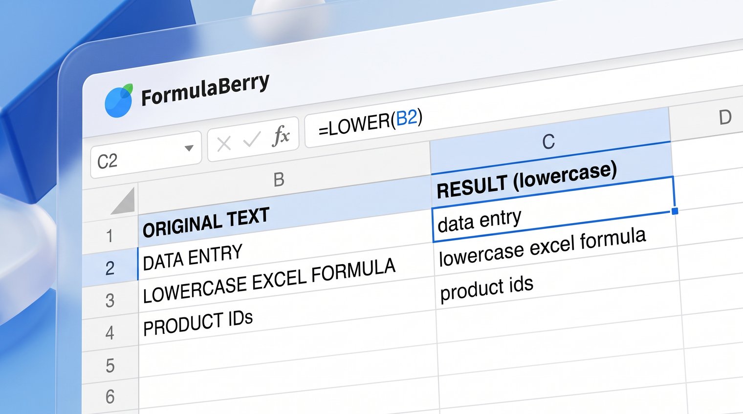
Enter LOWER with a cell reference

Most of the time, the text you want to convert is already in a worksheet cell. Rather than typing that text into the formula, point LOWER to the source cell.

• Click an empty cell next to the text you want to convert.
• Type =LOWER(A2), replacing A2 with the cell that contains your text.
• Press Enter.
• Check that the returned result has the lowercase text you expected.

The original text in A2 will not change. Excel displays the converted result in the cell containing the formula. This is useful because you can review the cleanup before replacing any original data.

Example: Convert one name or label to lowercase

Suppose cell A2 contains MONTHLY SALES REPORT. In B2, enter:

=LOWER(A2)

The result is monthly sales report. You can also enter text directly in the formula, such as =LOWER("MONTHLY SALES REPORT"), but a cell reference is the practical choice for spreadsheet cleanup.

Convert an entire range to lowercase by filling the formula down

To change capital letters to lowercase in Excel for a full list, write the formula once and fill it down. This works well for customer names, imported labels, email addresses, product descriptions, and other text columns.

Start in the first empty result cell beside your source data. If the original values begin in A2, enter =LOWER(A2) in B2 and press Enter. Then select B2 and use the small square at the lower-right corner of the cell, called the fill handle.

• Drag the fill handle down to the final row you need.
• Or, double-click the fill handle when the adjacent source column has a continuous list.
• Review a few formulas in the result column to make sure the references move row by row: A2, A3, A4, and so on.

A common mistake is double-clicking the fill handle when there are blanks in the source column. Excel may stop filling at the first break in the nearby data. In that situation, drag the fill handle over the intended range, or select the result range and fill the formula down manually.

Replace the original text with lowercase values when needed

A formula cannot overwrite the cell it reads from. Typing =LOWER(A2) into A2 creates a circular reference because Excel would be asked to calculate a cell from itself.

When you need the original column to contain lowercase text permanently, first create the results in a helper column. After reviewing them, replace the original values with copied results:

• Select the cells containing your LOWER formulas.
• Copy them with Ctrl+C.
• Select the original source range.
• Use Paste Special and choose Values.

This pastes the displayed lowercase text rather than the formulas. The source column is now lowercase, but the formulas are gone. Keep a backup column or duplicate the worksheet before pasting values, especially when cleaning business records or imported data you may need to audit later.

Keep formulas when the source text may change

Do not paste values if the original text is likely to be edited later. A LOWER formula updates automatically whenever its source cell changes, which makes a helper column useful for ongoing reports and cleanup workflows.

Label the new column clearly, such as Lowercase version. That makes it obvious which field is the original input and which one is the standardized output.

Use LOWER with other Excel functions for cleaner text

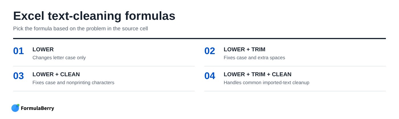
LOWER changes letter case only. If imported data also has extra spaces or hidden characters, combine LOWER with a focused cleanup function rather than expecting case conversion to fix everything.

Remove extra spaces with TRIM and LOWER

Use =LOWER(TRIM(A2)) when cells contain leading spaces, trailing spaces, or repeated spaces between words. For example, text such as MONTHLY SALES REPORT becomes monthly sales report.

TRIM is an effective default for ordinary spaces, but it does not remove every type of space copied from websites or external systems. In particular, nonbreaking spaces can remain even after using TRIM.

Clean nonprinting characters with CLEAN and LOWER

Use =LOWER(CLEAN(A2)) when imported text contains nonprinting characters, such as line-break-related characters from older exports or copied data. CLEAN removes supported nonprinting characters, and LOWER then standardizes the letter case.

When both spacing and nonprinting characters are causing trouble, use:

=LOWER(TRIM(CLEAN(A2)))

This is a sensible cleanup formula for many imported text fields. It removes common hidden characters, trims ordinary excess spaces, and converts letters to lowercase in one result.

Standardize email addresses cautiously

You can use =LOWER(A2) to create lowercase email addresses for consistent presentation or matching keys. For example, JANE.DOE@EXAMPLE.COM becomes jane.doe@example.com.

However, lowercasing an email address does not validate it. The local part before the @ symbol can technically be case-sensitive depending on the receiving system, even though many modern email services treat it as case-insensitive. Use lowercase normalization only when it fits the rules of the system where the data will be used.

Understand what LOWER does not change

LOWER does not alter numbers, punctuation, dates, cell formatting, or the original cell's contents. It only converts alphabetic characters in the text it returns.

For example, ABC-123 becomes abc-123, while 123 remains 123. A formula in the source cell is not rewritten, and applying LOWER to a cell does not change its font, color, or other formatting.

The result of LOWER is text. That matters when the output feeds a case-sensitive comparison, lookup process, export, or external workflow. For related formatting tasks, see the Excel TEXT formula guide. Be sure the next step expects a text value in lowercase rather than the original formatting or data type.

Change lowercase text to uppercase or proper case instead

LOWER is the correct function when every letter should be lowercase. If that is not your intended result, choose a different text function before filling a large range.

Use =UPPER(A2) for all capital letters. Use =PROPER(A2) for title-style capitalization, where the first letter of each word is capitalized.

Be careful with PROPER. It can produce unwanted results for acronyms, apostrophes, product names, and brand styling. For example, it may turn a carefully formatted company name into a version that looks polished but is incorrect.

Choose LOWER, UPPER, or PROPER based on the intended result

Using the source text mONTHLY sales report, the three functions return different results:

Formula	Result	Best use
=LOWER(A2)	monthly sales report	Standardized lowercase text
=UPPER(A2)	MONTHLY SALES REPORT	All-cap labels or codes
=PROPER(A2)	Monthly Sales Report	Simple title-style text

All three functions follow the same workflow: create the formula in a helper column, fill it down, and paste values only if you need to replace the original text permanently.

Fix common LOWER formula problems

If Excel displays =LOWER(A2) as text instead of returning a result, check whether an apostrophe appears before the equals sign. For example, '=LOWER(A2) tells Excel to treat the entry as text.

Cell formatting can cause the same problem. Change the cell format to General, click into the formula, and press Enter again. If the formula was entered while the cell was formatted as Text, simply changing the format may not be enough; you need to re-enter the formula.

If the result is lowercase but comes from the wrong row, inspect the cell reference. A formula in B2 should normally use A2, a formula in B3 should use A3, and so on. Incorrect references often happen when a formula is copied from a different table or when absolute references such as $A$2 are used unintentionally.

Another frequent issue is trying to convert text in place. LOWER must read from one cell and return the converted text in another cell. Use a helper column, then copy and paste values back over the original range if required.

Finally, regional Excel settings can affect formulas with multiple arguments. LOWER itself has one argument, so =LOWER(A2) works without a separator issue. But formulas such as nested text-cleaning formulas or other multi-argument functions may require semicolons instead of commas in some installations.

Make text lowercase in Excel with a repeatable cleanup workflow

Use =LOWER(A2) when you need lowercase text, then fill the formula down for the rest of the column. Keep the formula column when the source data may change, or copy the results and paste values when you need a permanent replacement.

If the data has more than a capitalization problem, use =LOWER(TRIM(A2)) for extra spaces or =LOWER(TRIM(CLEAN(A2))) for common imported-text cleanup. This keeps the task controlled: clean the issue you actually have instead of altering data blindly.

If you need to compare the cleaned results against other text, see the Excel Contains formula guide. To remove duplicate values after standardizing a column, use the DISTINCT Excel formula guide.

For help generating, explaining, or correcting a nested Excel or Google Sheets text formula, try FormulaBerry.